Market conditions, investor sentiment and disposition effect. An empirical study based on China's stock market
ABSTRACT
Using the transaction data of the stock market and financial data of listed companies from 2003 to 2021 in China, we explore the existence form of the disposition effect. Then, we combine the Bayesian learning process with the DSSW model to investigate the disposition effect's size and performance when market conditions differ from investors' irrational beliefs. We find the disposition effect in China is asymmetric V-shaped and negatively correlates with investor sentiment significantly. In addition, affected by sentiment, its performance is opposite in the bull market and bear market. The above research and conclusions have theoretical and practical significance for understanding the disposition effect, optimizing investors' decision-making, and strengthening the capital market infrastructure.
Keywords: Disposition effect; Investor sentiment; Irrational expectation; Speculative trading.
JEL classification: G11; G12; G14.
Condiciones del mercado, sentimiento del inversor y efecto de disposición. Estudio empírico basado en el mercado bursátil chino
RESUMEN
Utilizando los datos de transacciones del mercado de valores y los datos financieros de las empresas cotizadas de 2003 a 2021 en China, exploramos la forma de existencia del efecto de disposición. A continuación, combinamos el proceso de aprendizaje bayesiano con el modelo DSSW para investigar el tamaño y el rendimiento del efecto de disposición cuando las condiciones del mercado difieren de las creencias irracionales de los inversores. En China, el efecto de disposición tiene forma de V asimétrica y una correlación negativa significativa con el sentimiento de los inversores. Además, afectado por el sentimiento, su rendimiento es opuesto en el mercado alcista y en el mercado bajista. La investigación y las conclusiones anteriores tienen importancia teórica y práctica para comprender el efecto de disposición, optimizar la toma de decisiones de los inversores y reforzar la infraestructura del mercado de capitales.
Palabras clave: Efecto de disposición; Sentimiento del inversor; Expectativa irracional; Negociación especulativa.
Códigos JEL: G11; G12; G14.
1. Introduction
The disposition effect refers to investors' tendency to sell profitable investments and hold loss investments (Shefrin & Statman, 1984). Theory and practice have proved that it widely exists in the capital market in different countries and regions (Odean, 1998; Grinblatt & Keloharju, 2001; Vinokur, 2009). In addition, there is also much evidence that both individual and institutional investors have the disposition effect (Zahera & Bansal, 2019; Coval & Shumway (2005). It means the disposition effect has become one of the factors that cannot be ignored in asset pricing. The research on it is of great significance for pricing financial assets more accurately and making the prices better reflect the actual market situation.
However, the causes and motives of the disposition effect are still unclear. The rational person hypothesis could not explain it (Weber & Camerer, 1998; Auden, 1998). In addition, the prospect theory based on behavioural economics may also not explain the disposition effect. In the latest research, Ben David & Hirshleifer (2012) believe that investor beliefs could explain the disposition effect. We could divide investor beliefs into rational beliefs and irrational beliefs. Among them, investors with rational beliefs should constantly follow the Bayesian rule to update their rational beliefs (Zhang & Wang, 2013). Moreover, the irrational belief is equivalent to the investor sentiment proposed by Baker & Wurgler (2006).
Meanwhile, Black (1986) pointed out that there are a large number of irrational or bounded rational traders in the market, who have biased (non-Bayesian) beliefs about the future returns of risk assets, that is, investor sentiment (Baker & Wurgler, 2006). Investors' irrational beliefs (investor sentiment) play an essential role in asset trading behaviour and asset price formation (Antoniou et al., 2013; Dumas et al., 2009; Da et al., 2015). In theory, rational traders could correct the market mispricing caused by investor sentiment through arbitrage so that the market could recover effectively. However, asset mispricing is usually difficult to eliminate due to short selling, arbitrage restrictions and transaction costs in the actual situation.
The above phenomenon is evident in China's stock market. Chinese investors have a shorter average education period and lack investment experience, thus showing various irrational behaviours (herd effect, disposition effect, etc.). For example, China's capital market shows the characteristic of youth. In 2021, the average age of new investors was 30.4 years, 0.5 years lower than in 2019. Moreover, their investment decisions are also affected by securities analysts, and the stronger the commission relationship, the greater the deviation of analysts' forecasts (Wu et al., 2018). Yao et al. (2019) found the gambling atmosphere in China's stock market was intense, and the arbitrage restrictions further exacerbated it. Leverage trading not only does not ease the arbitrage restrictions but also causes abnormal price fluctuations (Peng & Hu, 2020). The above phenomena are mainly affected by individual investors' beliefs and sentiment mechanisms. In China, the proportion of individual investors is considerable. According to the disclosure of China Securities Depository and Clearing Co., Ltd., in October 2021, the number of active accounts of Chinese individual and institutional investors was about 157.09 million and 353000, respectively, with individual investors accounting for 97.78%. From the above, we believe irrational investors account for a relatively high proportion of China's stock market (compared with mature markets).
Meanwhile, the friction in China's stock market is more serious, which leads to more significant asset mispricing. There is also an apparent feature of speculation in China's stock market. The stock price fluctuates violently in a short time, which is easy to form large profits and losses. Speculators would use the deviation of individual investors' disposition effect to break the price away from the fundamentals (Geng & Lu, 2017). Moreover, speculation in China is contagious and would spread to the whole market (Liu et al., 2015). When the market cannot eliminate irrational investors, the investor group would deviate from rationality, which means the investors are irrational on average, and the overall irrational degree of Chinese investors is greater.
Investor sentiment has an essential impact on the disposition effect. In the previous literature, Ben-David & Hirshleifer (2012) believed that the renewal of investors' beliefs caused the disposition effect. Afterwards, Lee et al. (2013) measured the intensity of the disposition effect according to the market conditions (bull market and bear market). We believe that their result is driven by investor sentiment. Therefore, in our research, we further divide the stock market according to market status and investor sentiment to study the impact of belief renewal on the disposition effect. On the whole, we find investor sentiment and the disposition effect are negatively correlated. But in the sub-sample of the bull market, this relationship becomes positive. Specifically, when the stock price rises, they tend to sell stocks to obtain immediate income. And when the stock price decreases, due to their overconfidence and fluke, they think the decline is temporary, and the price would return to the expected state. Therefore, they tend to hold loss stocks in the hope of gaining profits in the future. Also, due to the psychology of profit-seeking and risk aversion, investors are more willing to realize profits rather than face losses, leading to the irrational behaviour of selling in the profit state and holding in the loss state, too. In the bull market, with the increase in investor sentiment, investors are more willing to hold profitable stocks, thus showing a strong disposition effect.
As the largest developing country, China's economic strength currently ranks second in the world. The capital market in China continues to open, and its scale continues to expand, with the total market value increasing from 2.8 billion CNY in 1990 to 80 trillion CNY in 2020. Therefore, taking China's capital market as the research object is conducive to the in-depth exploration of asset pricing in China, a vital economy, and provides some reference for the international community to study this field further. However, the research on the disposition effect, especially its manifestation, is still in its infancy in China. Meanwhile, most scholars use account transaction data to study the disposition effect. The obvious disadvantage of this method is that the sample period is usually short, which makes it difficult to describe the change of the disposition effect in the whole market. In addition, there are few studies on the relationship between investor sentiment and disposition effect, and they do not deeply understand the relationship and mechanism between investors' selling decisions and market conditions. Therefore, we make the following innovations to compensate for the above shortcomings. Firstly, we creatively adopt An's (2016) method to measure the disposition effect in China's stock market. Furthermore, we confirm again that it exists in an asymmetric V-shape. Secondly, we use the corporate financial data from 2003 to 2021 to study the disposition effect, which increases the sample size and could better describe China's stock market. Thirdly, we study the relationship between investor sentiment and disposition effect by multidimensional sort method. We found that investor sentiment and disposition effects are negatively correlated during the bear market while positively correlated during the bull market, which provides a new perspective for scholars in this field.
2. Literature review, theoretical models and hypothesis
2.1. Disposition effect and its explanation
In 1984, Shefrin & Statman first observed the disposition effect. They proposed it refers to the phenomenon that investors tend to sell profitable investments and hold loss investments. Subsequently, both traditional financial scholars and behavioural finance scholars try to explain this. Traditional financial scholars try to study it based on the average regression of stock prices (Andreassen, 1988), private information and portfolio adjustment theory (Lakonishok & Smidt, 1986). However, Weber & Camerer (1998) and Auden (1998) confirmed that traditional finance could not explain the disposition effect. Because according to the hypothesis of rational people, investors would continue to hold profitable stocks and sell loss-making stocks to maximize wealth. From the perspective of behavioural finance, scholars believe that the S-shaped utility curve (Kahneman & Tversky, 1979) could explain the disposition effect based on the investor sign realization preferences. Meanwhile, Weber & Camerer (1998) confirmed that the disposition effect is due to irrational cognition like loss aversion. However, many scholars found that the investor sign realization preferences could not fully explain the disposition effect and further put forward the discontinuous sale possibility curve (Kaustia, 2010), asymmetric V-shaped disposition effect (Ben David & Hirshleifer, 2012) and ranking effect (Hartzmark, 2015).
2.2. Areas and fields where the disposition effect exist
Since the disposition effect was discovered, many scholars have proved that it widely exists in different countries and regions. Odean (1998) found a disposition effect in the U.S. stock market, and Grinblatt & Keloharju (2001) also found it in the Polish stock market. It has also been confirmed in other countries and regions, such as the European Union (Vinokur, 2009), the United Kingdom (Richards & Rutterford et al., 2017), Macao (Chui, 2001), etc. According to the research of Genesove & Mayer (2001), Heath et al. (1999) and Locke & Mann (2005), the disposition effect also exists in the real estate market, options market and futures market and has an essential impact on these markets.
2.3. Influencing factors of the disposition effect
As for the influencing factors of the disposition effect, the existing literature mainly focuses on race, investor category and so on. Frino et al. (2015) found that the Chinese have a more substantial disposition effect on the Australian stock market. Coval & Shumway (2005) found that individual and institutional investors have apparent disposition effects. However, Zahera & Bansal (2019) believe it is more significant for individual investors because they are overconfident. Frydman & Wang (2020) found the more sensitive individual investors are to profits and losses, the more significant the disposition effect. In addition, loss aversion, investor maturity (Ahn, 2021), housing mortgage loans and shareholder loyalty programs (Brown et al., 2006) would also affect the disposition effect.
2.4.. Measurement of investor sentiment
Many scholars have studied the measurement of investor sentiment, among which the paradigm of Baker & Wurgler (2006) is the most classic and widely used. They use principal component analysis to get a more useful indicator of investor sentiment. In addition, scholars have also proposed other indexes, including turnover rate (Bandopadhyaya & Jones, 2006), the number of negative words (Tetlock, 2007), mutual fund flow (Ben-Rephael et al., 2012), overnight return rate (Aboody et al., 2018), etc. These indexes could predict the stock market (Tetlock, 2007; Huang et al., 2015). For example, McGurk et al. (2020) believe that investor sentiment significantly impacts abnormal stock returns. Da et al. (2015) found that investor sentiment indicators could predict market returns and capital flows. Sun et al. (2016) successfully predicted the S&P 500 index using the indicators.
2.5. Disposition effect of China's capital market
Chen et al. (2007) pointed out a significant disposition effect in China's stock market. Then, referring to the method of Odean (1998), Liu & Chen (2008) tested the inverted V-shaped structure of it. In addition, scholars also have studied the influencing factors of the disposition effect, including age, gender, investor category and so on. Chen et al. (2007) proposed when investors are older and hold investment products for a long time, the disposition effect would be more significant. Wu et al. (2018) found that the disposition effect of male investors is less than that of female investors, and that of young investors (under the age of 35) is weaker. According to the research of Zahera & Bansal (2019), the disposition effect of individual investors is more evident than institutional investors because they are more overconfident. Ni et al. (2015) found an apparent overreaction in the Chinese stock market by studying investor sentiment, which is a significant factor leading to incorrect pricing. Yang & Yang (2022) found more speculation in China's stock market because of the more significant proportion of individual investors. Lin et al. (2007) tested the trading behaviour of individual investors under different historical stock prices through psychological experiments. The results show that the longer the stock price rises, the more likely investors are to sell shares. In addition, the stock return would also impact the disposition effect. Zaiane (2013) believes that high returns may lead to investors' overconfidence and increase the disposition effect of China's stock market.
2.6. Existing form of the disposition effect
Odean (1998) and Kaustia (2010) found the disposition effect has an inverted V-shaped structure. In this structure, with the increase of profit and loss percentage, the possibility of selling decreases, which is the greatest at the breakeven point. Grinblatt & Han (2005) illustrated that the disposition effect is a symmetrical V-shaped structure through Capital Gain Overhang (CGO) construction. Ben David & Hirshleifer (2012) studied the U.S. stock market using individual investors' account data and confirmed the asymmetrical "V" shape. However, Calvet et al. (2009) analyzed the transaction data from Swedish and found the disposition effect is an asymmetric "V" structure. With the increase in profits and losses, the possibility of selling stocks also increases. An (2016) also found an asymmetric V-shaped disposition effect in the U.S. stock market using the proxy variable constructed by stock closing price and turnover rate. In short, scholars have no unified view on the existing form of disposition effect at present. Our research focuses on exploring whether the V-shaped form is symmetric or asymmetric. The two different forms are shown in Figure 1.
Figure 1. Symmetrical and Asymmetrical V-shaped Selling Propensity in Response to Profits
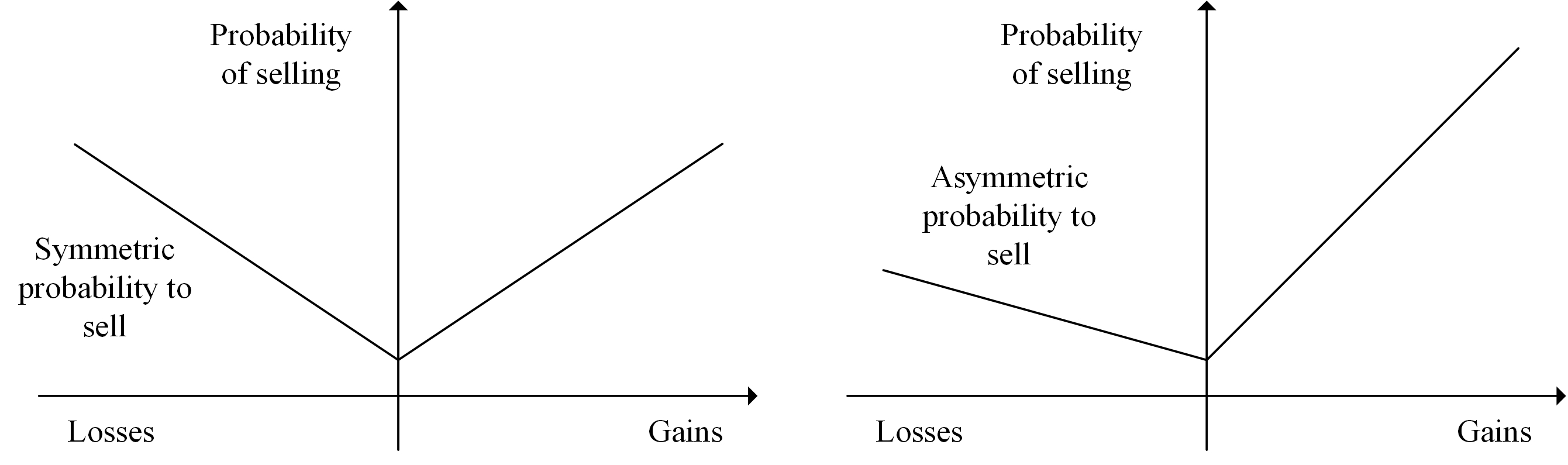
Figure 1. Symmetrical and Asymmetrical V-shaped Selling Propensity in Response to Profits. The left graph is a symmetrical V-shaped disposition effect. It was expressed by Ben David & Hirshleifer (2012) by constructing the proxy variable CGO. It means the selling probability caused by unrealized gains and unrealized losses is the same. The right graph is an asymmetric disposition effect. It was expressed by An (2016) by constructing the proxy variable VNSP. It means the probability of selling due to unrealized gains is greater.
Ben David & Hirshleifer (2012) believed that the belief change caused the V-type disposition effect. That is, when the stock price falls, the selling probability of the stock increases, which may be due to the renewal of beliefs (rational or irrational beliefs). In the study of the form of the disposition effect in China, we adopt the latest method of An (2016). Therefore, based on the above discussion, we infer that belief renewal would produce the V-shaped disposition effect. Moreover, after testing through An's method, we would reach the same conclusion as him. This is our hypothesis 1, and its specific expression is as follows.
H1: In China's stock market, the disposition effect is asymmetric V-shaped.
2.7. Investor sentiment and its impact on the disposition effect
Baker et al. (2012) pointed out that the definition of investor sentiment is still vague. A widely accepted explanation comes from Lee et al. (1990). They believe that investor sentiment refers to the deviation between the expected price (based on investors' beliefs and value judgments) and the actual price of financial products. Although the prospect theory (Kahneman & Tversky, 1979) and its extension, such as narrow framing, probability weight function, whether profits and losses are realized, etc. (Barberis & Huang, 2008); (Barberis & Xiong, 2009) discussed the influence of investor preference and analyzed how it affects the selling decision, they fail to reflect the impact of investors' beliefs on the disposition effect (Barberis & Huang, 2008). Later, much literature has proved that investors' irrational beliefs (investor sentiment) play an essential role in asset trading and price formation (Antoniou et al., 2013; Dumas et al., 2009; Da et al., 2015). For example, Kajol et al. (2020) used Social Network Analysis (SNA) to analyze the factors affecting the disposition effect. The study found that social trust and investor sentiment are the two most important.
Ben David & Hirshleifer (2012) found that the intensity of the disposition effect of individual investors is related to their trading frequency, gender, speculation and other characteristics. In other words, this is the result of irrational belief renewal. Then, Zhang & Wang (2013) combined the DSSW model with the Bayesian learning process to build a theoretical model to study the relationship between irrational beliefs and investor sentiment. A noticeable feature in China's stock market is that there are speculative activities, and investors' financial literacy and investment experience are low. Therefore, we believe that the renewal of irrational beliefs causes the disposition effect in China's stock market. Moreover, investor sentiment could be an indicator to measure irrational beliefs. That is, the size and intensity of the disposition effect would be significantly affected by it. Therefore, we propose hypothesis 2.
H2: Investor sentiment is negatively correlated with the disposition effect. The higher the investor sentiment, the weaker the disposition effect.
Many scholars have found that the degree of investor disposition effect is significantly different in different market conditions. For example, Lehenkari & Perttunen (2004) found that the probability of selling loss stocks may be higher than the probability of selling profit stocks due to the increase of the number of loss-making stocks in the portfolio in a falling market, so the disposition effect becomes weak, and the disposition effect is evident in a rising market or a stable market. By taking the bull and bear markets as the proxy variable of subjective belief, Cheng et al. (2013) studied the relationship between subjective belief and the intensity of the disposition effect and found that the disposition effect is more substantial in the bear market. In other words, subjective belief impacts the disposition effect, and when the market belief is small, the strength of the disposition effect is large. This evidence shows that investors' selling decisions are sensitive to the market state, but the direction of influence is inconsistent, and the academic community has not yet profoundly understood the impact mechanism behind it.
Furthermore, Thornton (2021) found a positive correlation between investor sentiment and the disposition effect. Investors with low sentiment would think about their decisions systematically. It shows that they are more willing to hold profitable stocks, which would reduce the disposition effect. However, even in different market states, investors will not only consider the historical stock price trend (market condition) but also be affected by the belief formed by the expectation of future cash flow and investment risk (investor sentiment). Chinese investors are highly irrational, which would show a high fluctuation of investor sentiment. Therefore, we infer that when market conditions are consistent with investor sentiment, the disposition effect would be amplified due to insufficient information response. When they are inconsistent, investors will overreact, thus reducing the disposition effect. Therefore, based on the hypothesis 2, we further assume the disposition effect of China's stock market ranks.
H3: During the bear market, the disposition effect of depressed investors is the largest. However, in the bull market, this is the smallest. Specifically, the assumption could be divided into the following four situations.
Market conditions are the same as investor sentiment:(1) Bull market-High sentiment. (2) Bear market-Low sentiment.
Market conditions are different from investor sentiment:(1) Bear market-High sentiment. (2) Bear market-Low sentiment.
3. Methodology and data
3.1. Core indicators construction
In this part, we describe the construction of the core variables. On the one hand, we use the latest method to construct the proxy variable of the disposition effect. One of the advantages is the use of macro data, which makes the results more robust and reproducible. On the other hand, On the construction of investor sentiment indicators, we use the classic approach of Baker & Wurgler (2006) to construct investor sentiment indicator, which could make our results more credible.
3.1.1. Construction of the disposition effect
A common method to construct the disposition effect indicator is to build the unrealized gain (Gain) and unrealized loss (Loss) proposed by An (2016). We use public data, such as monthly turnover rate (V) and closing price of stocks on that day (P) construct the above two indicators. In contrast, most scholars use personal account data. We observe that the period of such samples is short, which would affect the robustness of the results. At the same time, personal account data is non-public and difficult to obtain, so the relevant researches are almost impossible to copy. In addition, the data are usually provided by securities companies. The single data source may lead to bias in the overall estimation. Therefore, we use public data for the indicator construction to compensate for the above deficiencies. On the one hand, the data's openness could increase our results' replicability and help other scholars conduct in-depth research. On the other hand, data availability could make our research's period larger and the results more robust. Based on the above analysis, we use the monthly closing price and turnover rate of stocks at time 𝑡−60 (five years ago) to measure the unrealized return of investors at time 𝑡,o as to evaluate the Gain. Loss is constructed in the same way. The specific constructions are as follows:
\[\begin{equation} \label{eq1} \small Gain_{t} = \sum_{n = 1}^{N}{W_{t - n}* gain_{t - n}} \ \ \ \ \ (1) \end{equation}\] \[\begin{equation} \label{eq2} \small gain_{t - n} = \frac{P_{t} - P_{t - n}}{P_{t}}\ \ \ \ \ \ \ (P_{t - n} \leq P_{t}) \ \ \ \ \ (2) \end{equation}\] \[\begin{equation} \label{eq3} \small Loss_{t} = \sum_{n = 1}^{N}{W_{t - n}*loss_{t - n}} \ \ \ \ \ (3) \end{equation}\] \[\begin{equation} \label{eq4} \small loss_{t - n} = \frac{P_{t} - P_{t - n}}{P_{t}}\ \ \ \ \ \ \ (P_{t - n} > P_{t}) \ \ \ \ \ (4) \end{equation}\] \[\begin{equation} \label{eq5} \small W_{t - n} = \frac{1}{k}V_{t - n}\prod_{i = 1}^{n - 1}{\lbrack 1 - V_{t - n + i}\rbrack} \ \ \ \ \ (5) \end{equation}\] \[\begin{equation} \label{eq6} \small k = \sum_{n}^{}V_{t - n}\prod_{i = 1}^{n - 1}{\lbrack 1 - V_{t - n + i}\rbrack} \ \ \ \ \ (6) \end{equation}\]Where, \(V_{t - n + i}\) is the monthly turnover rate of each stock, \(P_{t}\) is the closing price of the stock on that day, \(W_{t - n}\) represents the proportion of stocks purchased but not sold on the day (t-n), and (n-1) is the total trading days of the previous five years.
3.1.2. Construction of investor sentiment
Referring to the indicators and principal component analysis method used by Baker & Wurgler (2006) and taking into account the unique situation of China's stock market and the availability of data, we select closed-end fund discount rate (ECEFD), IPO scale (EIPON), IPO first-day return (ERIPO), market turnover rate (ET) and the number of new investors (ENIA) to measure investor sentiment. Specifically, we use these five indicators and their first-order lag for principal component analysis and select the indicators with the high contribution. Then, the consumer price index (CPI), producer price index of industrial products (PPI) and macroeconomic business index (MBI) are processed to eliminate the influence of macro factors. Finally, we analyze the residual and get the investor sentiment index. The corresponding regression results are shown in tables (1)-(7) in the appendix. Furthermore, the calculation formula of the investor sentiment indicator we finally obtain is as follows:
\[\begin{equation} \label{eq7} \small \begin{split} Senti_{t} =&\ 0.2369 \times ECEFD_{t} + 0.1883 \times EIPON_{t} \\ & + 0.2164 \times ERIPO_{t - 1} - 0.0779 \times ET_{urnover,\ t - 1}\\ & + 0.1466 \times ENIA_{t - 1} \end{split} \ \ \ \ \ (7) \end{equation}\]3.2. Explanatory variables, explained variables and control variables
We choose the return of each stock at time\(\ (\)t+1\()\) as the explained variable. The core explanatory variables include symmetrical disposition effect proxy variable CGO and asymmetric disposition effect proxy variable VNSP. And the CGO is a proxy variable of the symmetrical V-shaped disposition effect. It is derived from Girnblatt & Han (2005) and consists of unrealized gains and unrealized losses with equal weight. We use it to test whether the form of the disposition effect is symmetrical. Its specific form is shown in equation (8). The construction of VNSP (asymmetric V-shaped Net Selling Property) is based on the method of An (2016). Specifically, it is the gain and loss coefficient ratio after controlling all variables. In the following article, we adopt the same method as An (2016) to obtain the VNSP of China's stock market. The specific results will be discussed in section 4.2. In addition, the definitions and sources of all relevant variables are shown in Table 1 below.
\[\begin{equation} \label{eq8} \small CGO_{t} = Gain_{t} + Loss_{t} \ \ \ \ \ (8) \end{equation}\]Table 1. Variables Definition and the Sources
| Variable | Definition | Source |
|---|---|---|
| Ret | One-month ahead excess stock returns. | CSMAR |
| Gain | Measure the degree of "unrealized" profitability of most stock investors; see An (2016). | Derived from equation (1) |
| Loss | Measuring the extent of "unrealized" losses for most stock investors; see An (2016). | Derived from equation (3) |
| CGO | The proxy variable for the uniform binary monotonic disposition effect is derived from Gain and Loss. | Derived from equation (8) |
| VNSP | For asymmetric V-shaped Net Selling Propensity, see Ben David & Hirshleifer (2012). | Derived from equation (22) |
| Senti | For an indicator of investor sentiment in the Chinese stock market, see Baker & Wurgler (2006). | Derived from equation (7) |
| \(\small{ Ret_{t-1} }\) | Represents the return of the stock in the month (t-1), which is used to control the short-term reversal effect. | Constructed on desk |
| \(\small{ Ret_{t-12,t-2}}\) | Represents the cumulative return of the stock from the month (t-12) to month (t-2), which is used to control the momentum effect. | Constructed on desk |
| \(\small{ Ret_{t-36,t-12} }\) | Represents the cumulative return of the stock from the month (t-36) to month (t-13), which is used to control the long-term reversal effect. | Constructed on desk |
| \(\small{ Ret_{t-12,t-2}^{+}}\) | The momentum effect of past positive returns, concerning Hong et al. (2000). The calculation formula is \(\small{ Ret_{t-12,t-2}^{+} = Max\{Ret_{t-12,t-2}, 0\} }\). | Constructed on desk |
| \(\small{ Ret_{t-12,t-2}^{-}}\) | The momentum effect of past negative returns, concerning Hong et al. (2000).The calculation formula is \(\small{ Ret_{t-12,t-2}^{-} = Min\{Ret_{t-12,t-2} ,0\} }\). | Constructed on desk |
| LnSize | The logarithm of the size of the listed company, which is measured by the circulating market value, see Luo et al. (2017) and Chen et al. (2019). | Constructed on desk |
| LnBM | Shows the log of the book-to-market ratio of the stock in month t, which is measured by the ratio of net assets per share to the closing price, see Luo et al. (2017) and Chen et al. (2019). | Constructed on desk |
| IVol | Idiosyncratic volatility is constructed using market, firm size, and book-to-market factors, see Ang et al. (2006). | Constructed on desk |
| Turn | Turnover rate. | CSMAR |
| Beta | the beta coefficient of the stock, according to Bali et al. (2011). | Constructed on desk |
| Leverage | (Long-term debt + short-term debt + minority interests + preferred stock)/total asset | Constructed on desk |
| Illiquidity | Illiquidity indicator, according to Amihud (2002). The calculation formula is \({ Illiquidity_{iy} = \frac{1}{D_{iy}} \sum_{t=1}^{D_{iy}} \frac{|R_{iyd}|}{VOLD_{iyd}} }\) | Derived from equation (8) |
Note: Where Diy is the number of days of stock i in year y; Riyd is the return of stock i on d day of year y; VOLDiyd is the corresponding daily transaction volume.
3.3. Description of samples and data
Considering the accuracy and availability, we select the public data in China Stock Market & Accounting Research Database (CSMAR) to collect the stock trading data, financial data and institutional investors' shareholding data of Chinese listed companies from January 2003 to March 2021 for index construction. In addition, we exclude companies outside Chinese Mainland, financial enterprises (due to the particularity of their financial statements), S.T. companies (S.T.: special treatment, which refers to specially processed stocks. This is also a warning of delisting risk), bankrupt companies and enterprises that omit more than 60% of relevant data. Finally, through the above screening, we obtain 474,676 observations. Tables 2 and 3 are the descriptive statistics and coefficients of the key indicators used in our paper.
Table 2. Summary Stats for Variables
| variable | mean | p50 | sd | skewness | p10 | p90 |
|---|---|---|---|---|---|---|
| Ret | 0.013 | 0.000 | 0.142 | 1.252 | -0.136 | 0.178 |
| Gain | 0.040 | 0.015 | 0.061 | 2.660 | 0.000 | 0.118 |
| Loss | -0.157 | -0.095 | 0.197 | -3.089 | -0.383 | -0.004 |
| CGO | -0.107 | -0.064 | 0.213 | -2.072 | -0.357 | 0.090 |
| VNSP | 0.094 | 0.074 | 0.070 | 2.602 | 0.034 | 0.178 |
| Senti | 0.001 | -0.140 | 0.576 | 1.131 | -0.632 | 0.888 |
| \(\small{ Ret_{t-1}}\) | 0.015 | 0.001 | 0.157 | 13.558 | -0.136 | 0.180 |
| \(\small{ Ret_{t-12,t-2}}\) | 0.178 | 0.000 | 0.702 | 4.709 | -0.376 | 0.917 |
| \(\small{ Ret_{t-36,t-12}}\) | -0.295 | -0.143 | 0.836 | -2.356 | -1.259 | 0.551 |
| \(\small{ Ret_{t-12,t-2}^{+}}\) | 0.299 | 0.000 | 0.626 | 6.260 | 0.000 | 0.915 |
| \(\small{ Ret_{t-12,t-2}^{-}}\) | 0.121 | 0.000 | 0.166 | -1.334 | 0.376 | 0.000 |
| LnSize | 8.283 | 8.251 | 1.253 | 0.340 | 6.718 | 9.812 |
| LnBM | -1.045 | -0.990 | 0.765 | -0.927 | -1.983 | -0.140 |
| IVol | 0.018 | 0.016 | 0.018 | 151.454 | 0.008 | 0.031 |
| Turn | 0.459 | 0.306 | 0.467 | 2.644 | 0.085 | 1.032 |
| Beta | 1.065 | 1.051 | 0.286 | 0.529 | 0.800 | 1.333 |
| Leverage | 0.478 | 0.482 | 0.215 | 2.065 | 0.191 | 0.745 |
| Illiquidity | 0.121 | 0.032 | 0.862 | 143.396 | 0.007 | 0.222 |
Table 3. Correlation Coefficient Table
| Ret | Gain | Loss | CGO | VNSP | Senti | \(\small{ Ret_{t-1} }\) | \(\small{ Ret_{t-12,t-2}}\) | \(\small{ Ret_{t-36,t-12}}\) | \(\small{ Ret_{t-12,t-2}^{+}}\) | \(\small{ Ret_{t-12,t-2}^{-}}\) | LnSize | LnBM | IVol | Turn | Beta | Leverage | Illiquidity | |
|---|---|---|---|---|---|---|---|---|---|---|---|---|---|---|---|---|---|---|
| Ret | 1.00 | |||||||||||||||||
| Gain | 0.09 | 1.00 | ||||||||||||||||
| Loss | 0.01 | 0.41 | 1.00 | |||||||||||||||
| CGO | 0.05 | 0.54 | 0.92 | 1.00 | ||||||||||||||
| VNSP | 0.07 | 0.48 | -0.61 | -0.41 | 1.00 | |||||||||||||
| Senti | 0.04 | 0.26 | 0.18 | 0.26 | 0.05 | 1.00 | ||||||||||||
| \(\small{ Ret_{t-1} }\) | 0.05 | 0.60 | 0.39 | 0.37 | 0.14 | 0.09 | 1.00 | |||||||||||
| \(\small{ Ret_{t-12,t-2}}\) | 0.02 | 0.27 | 0.23 | 0.30 | 0.02 | 0.54 | 0.02 | 1.00 | ||||||||||
| \(\small{ Ret_{t-36,t-12}}\) | -0.04 | -0.03 | -0.11 | -0.09 | 0.08 | -0.02 | -0.05 | -0.09 | 1.00 | |||||||||
| \(\small{ Ret_{t-12,t-2}^{+}}\) | 0.03 | 0.25 | 0.15 | 0.24 | 0.07 | 0.54 | 0.02 | 0.97 | -0.05 | 1.00 | ||||||||
| \(\small{ Ret_{t-12,t-2}^{-}}\) | -0.02 | 0.19 | 0.36 | 0.38 | -0.18 | 0.27 | 0.01 | 0.57 | -0.19 | 0.36 | 1.00 | |||||||
| LnSize | -0.10 | 0.12 | 0.02 | 0.04 | 0.09 | -0.07 | 0.02 | 0.05 | 0.09 | 0.02 | 0.14 | 1.00 | ||||||
| LnBM | 0.04 | -0.29 | -0.25 | -0.30 | -0.01 | -0.24 | -0.14 | -0.37 | -0.19 | -0.36 | -0.24 | -0.04 | 1.00 | |||||
| IVol | 0.01 | 0.37 | 0.14 | 0.24 | 0.18 | 0.28 | 0.29 | 0.27 | -0.01 | 0.28 | 0.07 | -0.10 | -0.30 | 1.00 | ||||
| Turn | 0.01 | 0.15 | 0.25 | 0.31 | -0.11 | 0.35 | 0.18 | 0.26 | -0.02 | 0.27 | 0.09 | -0.21 | -0.26 | 0.59 | 1.00 | |||
| Beta | -0.02 | -0.08 | -0.04 | -0.05 | -0.03 | -0.02 | -0.01 | -0.02 | -0.09 | 0.00 | -0.10 | -0.12 | 0.03 | 0.05 | 0.08 | 1.00 | ||
| Leverage | 0.02 | 0.02 | -0.03 | -0.02 | 0.05 | 0.03 | 0.01 | 0.04 | 0.02 | 0.05 | 0.00 | 0.02 | 0.12 | 0.03 | -0.01 | 0.04 | 1.00 | |
| Illiquidity | 0.05 | 0.04 | -0.12 | -0.10 | 0.15 | 0.01 | 0.02 | -0.03 | 0.00 | -0.01 | -0.07 | -0.22 | 0.03 | 0.02 | -0.05 | 0.01 | 0.02 | 1.00 |
3.4. Hypotheses testing
In this section, we tested hypothesis 1 using formula (9) and formula (11) constructed below. Firstly, we use unrealized gain (Gain) and unrealized loss (Loss) to test the form of the disposition effect empirically. Then, after controlling the relevant variables, we test whether \(Gain\) and \(Loss\) have an impact on the future earnings of stocks, and the specific model is as follows.
\[\begin{equation} \label{eq9} \small \begin{split} Ret_{i,t} =& \ \alpha + \beta_{1}Gain_{i,\ t - 1} + \beta_{2}Loss_{i,\ t - 1} + \beta_{3} Ret_{i,\ t - 1} + \beta_{4} LnSize_{i,\ t - 1}\\ & + \beta_{5} LnBM_{i,\ t - 1} + \beta_{6} Turn_{i,\ t - 1} + \beta_{7} Illiquidity_{i,\ t - 1}\\ & + \beta_{8} IVol_{i,\ t - 1} + \beta_{9} Beta_{i,\ t - 1} + \beta_{10} Leverage_{i,\ t - 1} \end{split} \ \ \ \ \ (9) \end{equation}\]Where, \(Ret_{i,t}\) is the return rate of each stock at time t, and \(Gain_{i,\ t - 1}\ \)and \(Loss_{i,\ \ t - 1}\) are the unrealized gain and unrealized loss at the time (t-1), respectively.
Secondly, we further test whether the asymmetric disposition effect exists. Therefore, we introduce the asymmetric disposition effect index (VNSP) to test whether it would invalidate the binary monotone disposition effect. Referring to the practice of An (2016), we use the monthly trading volume, closing price, and financial data of each stock screened to establish Gain and Loss through Fama-Macbeth regression and then determine VNSP. Next, VNSP and CGO are used to analyze the form of the disposition effect. An (2016) believes that the impact of investors' unrealized earnings on the future earnings of stocks is different from that of unrealized losses. And the greater the absolute value of the VNSP coefficient, the stronger the disposition effect. Specifically, he calculated the disposition effect of the U.S. stock market as follows.
\[\begin{equation} \label{eq10} \small VNSP_{USA} = Gain_{t} - 0.17Loss_{t} \ \ \ \ \ (10) \end{equation}\]Here, based on the method of Grinblatt & Han (2005), we use capital gain overhang (CGO) as a proxy variable for the binary monotone disposition effect. In addition, Grinblatt & Han (2005) constructed a theoretical model based on prospect theory and psychological explanation to explain why the disposition effect leads to the momentum effect. They believe that capital gain overhang (CGO) could absorb the impact of the momentum effect on stock future returns, so the impact of the momentum effect is not significant. So, would VNSP lead to the momentum effect? To solve this problem, we further test whether there is a binary monotone disposition effect in China's stock market and its relationship with the momentum effect. We introduce the first-order and twelfth-order lag of the return rate to control and test the reversal and momentum effects, respectively. The specific empirical model is constructed as follows.
\[\begin{equation} \label{eq11} \small \begin{split} Ret_{i,t} =& \ \alpha + \beta_{1}{VNSP}_{i,\ t - 1} + \beta_{2} CGO_{i,\ t - 1} + \beta_{3} Ret_{i,\ t - 1}\\ & + \beta_{4} Retail_{i,\ t - 1} + \beta_{5} LnSize_{i,\ t - 1} + \beta_{6} LnBM_{i,\ t - 1}\\ & + \beta_{7} Turn_{i,\ t - 1} + \beta_{8} Illiquidity_{i,\ t - 1} + \beta_{9} IVol_{i,\ t - 1}\\ & + \beta_{10} Beta_{i,\ t - 1} + \beta_{11} Leverage_{i,\ t - 1} + \beta_{12} Ret_{i,\ t - 12} \end{split} \ \ \ \ \ (11) \end{equation}\]Based on hypothesis 2, we assume that the disposition effect would be affected by investors' irrational beliefs (which could be considered as investor sentiment). In other words, we hope to explore the difference in the disposition effect when investor sentiment differs. In order to achieve this objective, we use the double-sorting test method. Specifically, we divided the sample into three sub-samples according to the size of investor sentiment: high (67%-100%), medium (33%-67%) and low (0%-33%), and each level of VNSP, Gain and Loss of are calculated respectively.
Then, we hope to study the disposition effect's intensity when market conditions differ from investor sentiment. So, in the following content, we take the bull and bear markets as market condition indicators and use the data from China's stock market to conduct an empirical study on the relationship between investor sentiment and disposition effect.
4. Empirical research
4.1. Estimation of the disposition effect
We use formula (9) to study the existing form of the disposition effect in China's stock market, and the regression results are shown in Table 4. Regression (1) is the impact of Gain and Loss on future earnings. We could find the results are both significant. However, Grinblatt & Han (2005) and Ben David & Hirshleifer (2012) believe the momentum and reversal effects would affect the disposition effect. Therefore, in regression (3), we control the short-term reversal effect (\(Ret_{t - 1}\)), long-term reversal effect (\(Ret_{t - 36,\ t - 12}\)), and add momentum effect (\(Ret_{t - 12,\ t - 2}\)) in regression (4). According to the research results of Hong et al. (2000), in the momentum effect, the positive and negative effects of past returns on future stock returns are different. So, we control \(Ret_{t - 12,t - 2}^{+}\) and \(Ret_{t - 12,t - 2}^{-}\) instead of \(Ret_{t - 12,\ t - 2}\) in regression (5). The results show that these two control variables are significant, indicating they significantly affect the disposition effect. And in this process, Gain and Loss increase significantly. Similarly, regression (6) and (7) add all the control variables, but the former does not add Illiquidity. We find the results of Gain and Loss are also significant in the two regressions. Through regression (4), it could be concluded that the disposition effect in China's stock market is asymmetric, and its specific form is:
\[\begin{equation} \label{eq12} \small VNSP_{China} = Gain_{t} - 0.34Loss_{t} \ \ \ \ \ (12) \end{equation}\]The coefficient -0.34 is the ratio of the regression results of Loss and Gain1, indicating the strength of the disposition effect. Compared with the result of 0.154 obtained by An (2016) in the U.S. stock market, the average value of V-shaped Net Selling Probability (VNSP) in China's stock market is much higher. It indicates the disposition effect of China's stock market is more obvious. It is consistent with the phenomenon we have observed: the proportion of individual investors in China is higher, the age is younger, and the financial literacy is lower. Due to these irrational beliefs, the disposition effect would be stronger.
Table 4. Impact of Unrealized Gain and Loss on Future Stock Returns (1)
| (1) | (2) | (3) | (4) | (5) | (6) | (7) | |
|---|---|---|---|---|---|---|---|
| Gain | 0.034*** | 0.045*** | 0.146*** | 0.155*** | 0.154*** | 0.213*** | 0.212*** |
| (5.620) | (7.452) | (15.050) | (15.970) | (15.858) | (22.394) | (22.320) | |
| Loss | -0.060*** | -0.054*** | -0.063*** | -0.053*** | -0.057*** | -0.052*** | -0.056*** |
| (-37.737) | (34.141) | (-27.623) | (-22.425) | (-25.135) | (-21.367) | (-23.871) | |
| LnSize | -0.013*** | -0.012*** | -0.012*** | -0.011*** | -0.011*** | ||
| (-37.405) | (-31.663) | (-32.473) | (-23.323) | (-23.817) | |||
| LnBM | 0.013*** | 0.009*** | 0.009*** | 0.008*** | 0.009*** | ||
| (22.869) | (15.691) | (16.251) | (14.935) | (15.458) | |||
| IVol | -0.253*** | -0.212*** | -0.187*** | -0.050 | -0.025 | ||
| (-4.439) | (-3.732) | (-3.283) | (-0.878) | (-0.446) | |||
| Turn | -0.016*** | -0.016*** | -0.016*** | -0.015*** | -0.015*** | ||
| (-12.768) | (-12.659) | (-12.525) | (-11.532) | (-11.369) | |||
| \(\small{ Ret_{t-1} }\) | -0.021*** | -0.038*** | -0.035*** | -0.034*** | -0.032*** | ||
| (-5.992) | (-10.690) | (-10.109) | (-9.645) | (-9.074) | |||
| \(\small{ Ret_{t-12,t-2}}\) | -0.014*** | -0.014*** | |||||
| (-17.215) | (-17.128) | ||||||
| \(\small{ Ret_{t-36,t-12}}\) | -0.001* | -0.003*** | -0.002*** | -0.002*** | -0.002*** | ||
| (-1.793) | (-5.938) | (-4.712) | (-5.430) | (-4.199) | |||
| \(\small{ Ret_{t-12,t-2}^{+}}\) | -0.016*** | -0.011*** | -0.011*** | ||||
| (22.438) | (-11.294) | (-11.150) | |||||
| \(\small{ Ret_{t-12,t-2}^{-}}\) | -0.025*** | -0.037*** | -0.036*** | ||||
| (13.834) | (-14.435) | (-14.363) | |||||
| Beta | -0.013*** | -0.013*** | -0.012*** | -0.011*** | -0.010*** | ||
| (-8.538) | (-8.606) | (-7.697) | (-7.259) | (-6.341) | |||
| Leverage | -0.000 | 0.000 | 0.000 | 0.001 | 0.001 | ||
| (-0.176) | (0.106) | (0.188) | (0.354) | (0.435) | |||
| Illiquidity | 0.020*** | 0.020*** | |||||
| (2.643) | (2.663) | ||||||
| Constant | -0.023*** | -0.026*** | 0.205*** | 0.192*** | 0.125*** | 0.106*** | 0.108*** |
| (-9.664) | (10.816) | (42.829) | (40.166) | (24.665) | (18.494) | (18.776) | |
| Ind | Yes | Yes | Yes | Yes | Yes | Yes | Yes |
| Year | Yes | Yes | Yes | Yes | Yes | Yes | Yes |
| N | 352370 | 352370 | 183602 | 183602 | 183334 | 180512 | 180244 |
| Adj. R2 | 0.050 | 0.055 | 0.075 | 0.078 | 0.077 | 0.083 | 0.083 |
| F | 487.785 | 494.948 | 320.068 | 314.535 | 315.854 | 311.567 | 313.291 |
Note: The explained variable is the excess stock return in period (t+1). * * *, * *, * respectively represent the significance at level of 1%, 5% and 10%.
In order to test the existence form of the disposition effect in China's stock market, we compare the symmetrical disposition effect CGO proposed by Grinblatt & Han (2005) with the VNSP obtained in this paper. Han believes that the existing form is a binary monotone, so the Gain and Loss have the same coefficient, and the coefficient of CGO is positive. Our results are shown in Table 5. Regression (1)-(6) are the results without VNSP. Among them, (1) and (2) control the momentum effect and its different forms, respectively. Regression (3) controls LnBM and IVol based on regression (1), and (4) further controls the different forms of momentum effect based on (3). Regressions (5) and (6) control Illiquidity based on regressions (3) and (4). The above is to test whether the disposition effect exists in the form of binary monotony. The CGO coefficients are significant but negative at the 1% significance level, showing no binary monotony disposition effect in China's stock market.
In regression (7)-(12), we add VNSP. Among them, (7) and (8) replace CGO with VNSP based on regression (3) and (4) to judge the existence form of the disposition effect preliminarily. (9)-(12) adopt the same control variable adjustment method as (3)-(6) to determine further whether there is an asymmetric V-shaped disposition effect. The results show that after adding VNSP to the regression, the coefficient of VNSP is significant at the 1% significance level. Moreover, the CGO coefficient becomes positive but not significant. It proves again that there is no monotonic binary but an asymmetric V-shape disposition effect in China's stock market.
Table 5. CGO VS VNSP
| (1) | (2) | (3) | (4) | (5) | (6) | (7) | (8) | (9) | (10) | (11) | (12) | |
|---|---|---|---|---|---|---|---|---|---|---|---|---|
| CGO | -0.027*** | -0.022*** | -0.023*** | -0.018*** | -0.014*** | -0.009*** | 0.0021 | 0.0021 | 0.0002 | 0.0039 | ||
| (-13.499) | (-10.506) | (-10.995) | (-8.382) | (-6.222) | (-3.923) | (0.28) | (0.28) | (0.03) | (0.53) | |||
| VNSP | 0.164*** | 0.156*** | 0.176*** | 0.180*** | 0.218*** | 0.222*** | ||||||
| (26.390) | (24.570) | (23.032) | (23.648) | (28.899) | (29.555) | |||||||
| LnSize | -0.010*** | -0.010*** | -0.010*** | -0.010*** | -0.008*** | -0.008*** | -0.012*** | -0.012*** | -0.012*** | -0.012*** | -0.011*** | -0.011*** |
| (-29.094) | (-28.142) | (-28.809) | (-27.876) | (-16.531) | (-16.094) | (-32.967) | (-31.896) | (-32.304) | (-33.225) | (-23.260) | (-23.788) | |
| LnBM | 0.009*** | 0.008*** | 0.008*** | 0.008*** | 0.010*** | 0.009*** | 0.010*** | 0.010*** | 0.009*** | 0.009*** | ||
| (15.597) | (14.789) | (14.294) | (13.498) | (16.951) | (16.065) | (16.794) | (17.488) | (16.000) | (16.645) | |||
| IVol | 0.172*** | 0.129** | 0.398*** | 0.356*** | -0.198*** | -0.213*** | -0.261*** | -0.234*** | -0.106* | -0.08 | ||
| (3.172) | (2.385) | (7.134) | (6.394) | (-3.545) | (-3.821) | (-4.586) | (-4.113) | (-1.847) | (-1.404) | |||
| Turn | -0.022*** | -0.022*** | -0.022*** | -0.022*** | -0.022*** | -0.023*** | -0.016*** | -0.016*** | -0.016*** | -0.016*** | -0.016*** | -0.015*** |
| (-21.021) | (-21.585) | (-17.835) | (-18.002) | (-16.646) | (-16.879) | (-12.480) | (-12.684) | (-12.776) | (-12.538) | (-11.994) | (-11.732) | |
| Beta | -0.013*** | -0.015*** | -0.012*** | -0.014*** | -0.010*** | -0.012*** | -0.012*** | -0.013*** | -0.013*** | -0.011*** | -0.011*** | -0.009*** |
| (-7.987) | (-9.245) | (-7.935) | (-9.116) | (-6.627) | (-7.851) | (-7.615) | (-8.614) | (-8.301) | (-7.299) | (-6.886) | (-5.888) | |
| Leverage | 0.004** | 0.003* | 0 | 0 | 0.001 | 0 | 0 | 0 | 0 | 0 | 0.001 | 0.001 |
| (1.996) | (1.715) | (0.160) | (0.032) | (0.363) | (0.235) | (0.205) | (0.107) | (0.165) | (0.261) | (0.427) | (0.519) | |
| \(\small{ Ret_{t-1} }\) | -0.021*** | -0.024*** | -0.021*** | -0.023*** | -0.009*** | -0.011*** | -0.038*** | -0.038*** | -0.044*** | -0.043*** | -0.037*** | -0.036*** |
| (-6.870) | (-7.684) | (-6.567) | (-7.206) | (-2.779) | (-3.448) | (-12.580) | (-12.490) | (-13.820) | (-13.479) | (-11.449) | (-11.120) | |
| \(\small{ Ret_{t-12,t-2}}\) | -0.017*** | -0.015*** | -0.015*** | -0.014*** | -0.015*** | -0.015*** | ||||||
| (-21.501) | (-17.491) | (-17.395) | (-17.551) | (-17.867) | (-17.845) | |||||||
| \(\small{ Ret_{t-36,t-12}}\) | -0.003*** | -0.004*** | -0.002*** | -0.003*** | -0.002*** | -0.002*** | -0.002*** | -0.003*** | -0.003*** | -0.002*** | -0.002*** | -0.002*** |
| (-6.827) | (-8.441) | (-4.334) | (-5.977) | (-3.771) | (-5.470) | (-4.648) | (-5.933) | (-5.862) | (-4.505) | (-5.354) | (-4.012) | |
| \(\small{ Ret_{t-12,t-2}^{+}}\) | -0.013*** | -0.010*** | -0.010*** | -0.011*** | -0.011*** | -0.011*** | ||||||
| (-13.249) | (-10.531) | (-10.253) | (-11.303) | (-11.535) | (-11.492) | |||||||
| \(\small{ Ret_{t-12,t-2}^{-}}\) | -0.048*** | -0.044*** | -0.044*** | -0.037*** | -0.039*** | -0.039*** | ||||||
| (-19.281) | (-17.409) | (-17.648) | (-14.762) | (-15.579) | (-15.397) | |||||||
| Illiquidity | 0.033*** | 0.032*** | 0.021*** | 0.022*** | ||||||||
| (3.220) | (3.198) | (2.660) | (2.680) | |||||||||
| Constant | 0.187*** | 0.110*** | 0.118*** | 0.188*** | 0.094*** | 0.091*** | 0.126*** | 0.192*** | 0.193*** | 0.128*** | 0.108*** | 0.110*** |
| -39.293 | -21.686 | -23.212 | -39.349 | -15.004 | -14.714 | -24.931 | -40.238 | -40.469 | -25.214 | -18.603 | -18.919 | |
| Ind | Yes | Yes | Yes | Yes | Yes | Yes | Yes | Yes | Yes | Yes | Yes | Yes |
| Year | Yes | Yes | Yes | Yes | Yes | Yes | Yes | Yes | Yes | Yes | Yes | Yes |
| N | 183674 | 183943 | 183334 | 183602 | 180244 | 180512 | 183334 | 183602 | 183602 | 183334 | 180512 | 180244 |
| adj. R2 | 0.072 | 0.073 | 0.073 | 0.074 | 0.077 | 0.078 | 0.077 | 0.078 | 0.078 | 0.077 | 0.084 | 0.083 |
| F | 319.737 | 320.931 | 311.572 | 311.842 | 304.063 | 304.415 | 320.491 | 320.169 | 313.696 | 314.224 | 312.112 | 313.137 |
Note: The explained variable is the excess stock return in period (t+1). * * *, * *, * respectively represent the significance at level of 1%, 5% and 10%.
4.2. Investor sentiment and the disposition effect: grouping test
We show the disposition effect under different investor sentiments in Table 6. Panel A is the intensity of the overall disposition effect, and Panel B specifically illustrates the strength by investigating the selling possibility of unrealized gain and loss, respectively. Next, the selection of control variables in all regression is based on regression (11) in Table 5. We find an apparent negative correlation between investor sentiment and the disposition effect. The higher the investor sentiment, the smaller the disposition effect. Investor sentiment represents investors' irrational expectations and beliefs about future stock returns, which would significantly affect investors' selling decisions, and then affect the degree of the disposition effect. Most irrational investors have not received professional investment training. They easily believe some gossip that has nothing to do with the stock price. It is also easy for them to blindly believe their judgment under the influence of external factors, thereby increasing their speculation to make profits quickly. If the stock price rises, irrational investors would think their previous information has been confirmed by the market and reflected in the stock price. Therefore, they are more willing to sell shares for
a profit. When the stock falls, they gradually think about whether their original decisions are correct. As the Loss continues to increase, they have to accept the fact that their initial judgment is wrong. Finally, their investment belief would change, and they may sell the stocks.
Table 6. Disposition Effects under Different Investor Sentiment Intensity
| Panel A | Panel B | |||||
|---|---|---|---|---|---|---|
| Sentiment | Sentiment | |||||
| Low | Middle | High | Low | Middle | High | |
| VNSP | 0.174*** | 0.159*** | 0.095*** | |||
| (17.638) | (17.211) | (6.583) | ||||
| Gain | 0.133** | 0.164*** | 0.166*** | |||
| (6.944) | (11.500) | (10.090) | ||||
| Loss | -0.063*** | -0.053*** | 0.033*** | |||
| (-17.654) | (-15.663) | (4.946) | ||||
| _cons | 0.178*** | 0.125*** | 0.279*** | 0.178*** | 0.125*** | 0.281*** |
| (16.450) | (16.724) | (26.159) | (16.464) | (16.656) | (26.392) | |
| Control | Yes | Yes | Yes | Yes | Yes | Yes |
| Ind | Yes | Yes | Yes | Yes | Yes | Yes |
| Year | Yes | Yes | Yes | Yes | Yes | Yes |
| N | 91772 | 115339 | 81862 | 91772 | 115339 | 81862 |
| adj. R2 | 0.217 | 0.150 | 0.102 | 0.217 | 0.150 | 0.104 |
| F | 335.073 | 282.905 | 171.599 | 327.336 | 276.180 | 171.463 |
Note: The explained variable is the excess stock return in period (t+1). * * *, * *, * respectively represent the significance at level of 1%, 5% and 10%.
4.3. Double sort of market state and investor sentiment
In order to further explore the relationship between investor sentiment and the disposition effect, we divide the market into two groups according to different market performances: bull market and bear market. Our division standard is the market average return judgment method. If the average market return minus the risk-free return is positive for at least three consecutive months, it is defined as a bull market, and the rest is a bear market (Cheng et al., 2013). Based on this, we further analyze the performance of investors' irrational beliefs and how they affect the strength of the disposition effect when the investor's mood is different from the market state. The specific results are shown in Table 7 and Table 8. We could find a negative correlation between investor sentiment and the disposition effect in a bear market. That is, in the bear market period, the higher the investor sentiment, the smaller the intensity of the disposition effect. However, investor sentiment and the disposition effect positively correlate in the bull market period. In addition, the results show the disposition effect is the largest in the bear market-low sentiment period (0.265, p<0.01) and the weakest in the bull market-low sentiment period (0.031, p>0.1). This result is generally consistent with our hypothesis 2. Our results could provide potential evidence for investor crowding trading behaviour. Furthermore, it confirms the view of Lee et al. (2013) that the disposition effect is more substantial during the bear market.
When in a bear market period, in the face of the decline of most stocks, optimistic investors are unwilling to immediately admit their original decision was wrong, or even subjectively shield the relevant bad news, because of the influence of previous cognition and judgment. However, with the deepening of stock losses, their willingness to sell would be stronger, but the intensity is relatively small. In contrast, according to the bad news, pessimistic investors would sell stocks more quickly. Therefore, the higher the investor sentiment in the bear market, the smaller the intensity of the disposition effect. In addition, we find that in the bear market period, the unrealized loss coefficient of investors with high sentiment is positive. The coefficient should be negative, which indicates investors do not seem to hold loss stocks at present (An, 2016; Han, 2005).
Most stocks rise during the bull market, making opportunists more confident and holding shares for a long time due to their positive expectations. We believe optimistic investors will continue to hold stocks after obtaining positive returns. And they would also continue to hold shares due to their optimistic expectations when they suffer losses. In contrast, pessimistic investors would also be cautious during the bull market, which shows they are more sensitive to the volatility of stock yield. We could find that investor sentiment in the bull market mainly affects investors' attitudes towards loss. Specifically, optimistic investors are more willing to hold lost assets, while pessimistic investors are on the contrary.
Table 7. Investor Sentiment and VNSP under Different Market Conditions
| Bull Market | Bear Market | |||||
|---|---|---|---|---|---|---|
| L | M | H | L | M | H | |
| VNSP | 0.031 | 0.116*** | 0.177*** | 0.265*** | 0.151*** | 0.079*** |
| (1.369) | (6.316) | (11.329) | (19.642) | (12.861) | (6.200) | |
| LnSize | -0.013*** | 0 | -0.021*** | -0.008*** | -0.011*** | -0.004*** |
| (-15.727) | (-0.496) | (-21.981) | (-11.315) | (-14.619) | (-3.313) | |
| LnBM | 0.010*** | 0.011*** | 0.013*** | 0.005*** | 0.009*** | 0.013*** |
| (7.346) | (10.967) | (8.370) | (4.053) | (7.881) | (6.899) | |
| IVol | 1.460*** | -0.294*** | -0.258* | 0.950*** | 0.259** | -1.103*** |
| (10.679) | (-2.722) | (-1.950) | (7.991) | (2.223) | (-5.715) | |
| Turn | -0.001 | 0.007*** | -0.032*** | -0.035*** | -0.015*** | 0.035*** |
| (-0.270) | (2.992) | (-12.408) | (-10.182) | (-5.685) | (11.637) | |
| \(\small{ Ret_{t-1} }\) | -0.216*** | -0.056*** | 0.01 | -0.134*** | -0.162*** | -0.106*** |
| (-23.678) | (-7.410) | (1.239) | (-16.260) | (-18.428) | (-9.732) | |
| \(\small{ Ret_{t-12,t-2}^{+}}\) | -0.008** | -0.028*** | -0.010*** | 0.028*** | 0.031*** | 0.015*** |
| (-2.268) | (-9.434) | (-6.605) | (7.571) | (11.173) | (7.913) | |
| \(\small{ Ret_{t-12,t-2}^{-}}\) | 0.051*** | -0.080*** | -0.002 | 0.054*** | 0.047*** | 0.112*** |
| (8.237) | (-18.554) | (-0.351) | (9.976) | (8.979) | (9.440) | |
| \(\small{ Ret_{t-36,t-12}}\) | 0.002 | 0.002*** | -0.012*** | 0 | -0.009*** | -0.001 |
| (1.568) | (2.634) | (-10.678) | (0.010) | (-11.014) | (-0.654) | |
| Beta | -0.002 | -0.009*** | -0.021*** | -0.021*** | -0.010*** | -0.016*** |
| (-0.563) | (-3.141) | (-4.774) | (-6.525) | (-3.280) | (-3.195) | |
| Leverage | -0.006 | 0.015*** | 0.001 | -0.014*** | -0.006 | 0.004 |
| (-1.503) | (5.083) | (0.146) | (-4.038) | (-1.635) | (0.671) | |
| Illiquidity | 0.087*** | 0.093*** | -0.001 | 0.153*** | 0.056*** | 0.014 |
| (4.702) | (3.56) | (-0.136) | (11.000) | (4.467) | (1.001) | |
| Constant | 0.085*** | 0.020** | 0.272*** | 0.064*** | 0.226*** | 0.068*** |
| (7.716) | (2.314) | (22.046) | (6.608) | (22.126) | (4.712) | |
| Ind | Yes | Yes | Yes | Yes | Yes | Yes |
| Year | Yes | Yes | Yes | Yes | Yes | Yes |
| N | 25307 | 41479 | 39076 | 24479 | 36558 | 16703 |
| adj. R2 | 0.362 | 0.175 | 0.083 | 0.113 | 0.204 | 0.324 |
| F | 404.324 | 166.34 | 113.302 | 88.124 | 224.999 | 246.516 |
Note: The explained variable is the excess stock return in period (t+1). * * *, * *, * respectively represent the significance at level of 1%, 5% and 10%.
Table 8. Investor Sentiment and Gain and Loss under Different Market Conditions
| Bull Market | Bear Market | |||||
|---|---|---|---|---|---|---|
| L | M | H | L | M | H | |
| Gain | 0.110*** | 0.120*** | 0.159*** | 0.245*** | 0.217*** | 0.107*** |
| (4.091) | (6.190) | (8.408) | (7.463) | (10.074) | (4.102) | |
| Loss | -0.067*** | -0.013*** | -0.031*** | -0.054*** | -0.094*** | 0.050*** |
| (-12.034) | (-2.731) | (-3.378) | (-12.953) | (-18.616) | -5.633 | |
| LnSize | -0.012*** | -0.001 | -0.021*** | -0.008*** | -0.010*** | -0.005*** |
| (-15.496) | (-1.216) | (-21.952) | (-11.114) | (-13.766) | (-4.531) | |
| LnBM | 0.009*** | 0.012*** | 0.013*** | 0.004*** | 0.008*** | 0.018*** |
| (6.465) | (11.754) | (8.345) | (3.561) | (7.317) | (9.186) | |
| IVol | 1.524*** | -0.396*** | -0.263** | 1.000*** | 0.305*** | -1.242*** |
| (11.055) | (-3.539) | (-1.986) | (8.287) | (2.593) | (-6.051) | |
| Turn | -0.001 | 0.008*** | -0.032*** | -0.035*** | -0.015*** | 0.037*** |
| (-0.169) | (3.229) | (-12.380) | (-10.273) | (-5.763) | (12.143) | |
| \(\small{ Ret_{t-1} }\) | -0.200*** | -0.079*** | 0.008 | -0.124*** | -0.151*** | -0.179*** |
| (-19.602) | (-9.785) | (0.927) | (-13.571) | (-15.361) | (-14.143) | |
| \(\small{ Ret_{t-12,t-2}^{+}}\) | -0.007* | -0.029*** | -0.010*** | 0.029*** | 0.031*** | 0.014*** |
| (-1.858) | (-9.948) | (-6.622) | (7.735) | (11.317) | (7.224) | |
| \(\small{ Ret_{t-12,t-2}^{-}}\) | 0.057*** | -0.085*** | -0.003 | 0.056*** | 0.049*** | 0.085*** |
| (8.785) | (-19.396) | (-0.442) | (10.152) | (9.185) | (7.144) | |
| \(\small{ Ret_{t-36,t-12}}\) | 0.001 | 0.002** | -0.012*** | 0 | -0.009*** | 0 |
| (1.461) | (2.292) | (-10.661) | (0.024) | (-10.923) | (-0.248) | |
| Beta | -0.002 | -0.008*** | -0.021*** | -0.022*** | -0.010*** | -0.012** |
| (-0.704) | (-2.894) | (-4.756) | (-6.634) | (-3.454) | (-2.369) | |
| Leverage | -0.006 | 0.015*** | 0.001 | -0.014*** | -0.006* | 0.005 |
| (-1.561) | (5.037) | (0.173) | (-4.081) | (-1.657) | (0.852) | |
| Illiquidity | 0.084*** | 0.097*** | 0 | 0.153*** | 0.056*** | 0.012 |
| (4.578) | (3.811) | (-0.024) | (10.978) | (4.47) | (0.863) | |
| Constant | 0.081*** | 0.026*** | 0.273*** | 0.063*** | 0.223*** | 0.070*** |
| (7.291) | (2.963) | (22.035) | (6.443) | (21.554) | (4.829) | |
| Ind | Yes | Yes | Yes | Yes | Yes | Yes |
| Year | Yes | Yes | Yes | Yes | Yes | Yes |
| N | 25307 | 41479 | 39076 | 24479 | 36558 | 16703 |
| adj. R2 | 0.362 | 0.176 | 0.083 | 0.113 | 0.204 | 0.33 |
| F | 395.535 | 162.816 | 110.249 | 85.867 | 219.225 | 238.654 |
Note: The explained variable is the excess stock return in period (t+1). * * *, * *, * respectively represent the significance at level of 1%, 5% and 10%.
5. Robustness test
We change the key indicators to ensure the reliability of our conclusions. Using the data of the past three years, we construct different Gain, Loss, and VNSP to replace the disposition effect indicators. In addition, we use the method of Ben-Rephael et al. (2012) to construct a different investor sentiment indicator. The construction principle is the same as that of Barker & Wurgler (2006). Specifically, it uses the average discount rate of closed-end funds, the average return on the first day of the IPO, the number of publicly issued shares in the current month, the market turnover rate, and the number of new opening accounts. After analysis, we could still get roughly the same results, which are robust (Table 9 and Table 10).
Table 9. Robustness Test for VNSP
| Bull Market | Bear Market | |||||
|---|---|---|---|---|---|---|
| L | M | H | L | M | H | |
| VNSP | 0.053*** | 0.185*** | 0.186*** | 0.218*** | 0.117*** | 0.055*** |
| (4.245) | (9.763) | (10.145) | (16.120) | (8.867) | (2.985) | |
| LnSize | -0.014*** | -0.001 | -0.021*** | -0.006*** | -0.005*** | -0.001 |
| (-9.530) | (-0.644) | (-21.625) | (-5.145) | (-5.901) | (-1.425) | |
| LnBM | 0.008*** | 0.011*** | 0.014*** | 0.002 | 0.002** | 0.009*** |
| (4.647) | (10.936) | (9.673) | (1.606) | (2.060) | (6.815) | |
| IVol | 1.177*** | 0.046 | -0.01 | 1.141*** | 0.346*** | -1.524*** |
| (7.101) | (0.438) | (-0.072) | (8.261) | (2.781) | (-10.506) | |
| Turn | -0.027*** | -0.004* | -0.029*** | -0.020*** | -0.003 | 0.021*** |
| (-5.790) | (-1.666) | (-10.929) | (-5.089) | (-0.905) | -7.997 | |
| \(\small{ Ret_{t-1} }\) | -0.156*** | -0.011 | 0.01 | -0.107*** | -0.195*** | -0.031*** |
| (-14.039) | (-1.535) | -1.221 | (-11.640) | (-20.511) | (-3.760) | |
| \(\small{ Ret_{t-12,t-2}^{+}}\) | -0.017*** | 0 | -0.012*** | 0.023*** | 0.012*** | 0.016*** |
| (-4.143) | (-0.097) | (-6.832) | (5.612) | (4.230) | (8.575) | |
| \(\small{ Ret_{t-12,t-2}^{-}}\) | 0.104*** | -0.137*** | 0.082*** | 0.059*** | 0.051*** | 0.080*** |
| (13.031) | (-32.110) | (10.870) | (9.246) | (9.639) | (12.412) | |
| \(\small{ Ret_{t-36,t-12}}\) | 0.007*** | 0.004*** | -0.011*** | -0.008*** | -0.003*** | -0.006*** |
| (4.338) | (4.859) | (-9.244) | (-6.374) | (-4.322) | (-5.172) | |
| Beta | 0.001 | -0.005* | -0.022*** | -0.009** | -0.010*** | -0.011*** |
| (0.126) | (-1.903) | (-5.266) | (-2.238) | (-3.333) | (-3.024) | |
| Leverage | -0.001 | 0.007** | 0.007* | -0.017*** | -0.008** | 0.003 |
| (-0.113) | (2.319) | (1.658) | (-4.163) | (-2.300) | (0.808) | |
| Illiquidity | 0.041** | 0.022 | 0.013 | 0.123*** | 0.057*** | 0.021 |
| (2.035) | (1.219) | (1.322) | (8.692) | (4.552) | (1.541) | |
| Constant | 0.248*** | 0.073*** | 0.306*** | 0.023* | 0.240*** | 0.087*** |
| (14.793) | (6.670) | (24.353) | (1.804) | (21.480) | (5.949) | |
| Ind | Yes | Yes | Yes | Yes | Yes | Yes |
| Year | Yes | Yes | Yes | Yes | Yes | Yes |
| N | 18339 | 48122 | 37402 | 19215 | 33435 | 23999 |
| adj. R2 | 0.18 | 0.189 | 0.115 | 0.142 | 0.198 | 0.274 |
| F | 72.148 | 303.739 | 133.419 | 89.817 | 178.416 | 229.621 |
Note: The explained variable is the excess stock return in period (t+1). * * *, * *, * respectively represent the significance at level of 1%, 5% and 10%.
Table 10. Robustness Test for Gain and Loss
| Bull Market | Bear Market | |||||
|---|---|---|---|---|---|---|
| L | M | H | L | M | H | |
| Gain | 0.002 | 0.060*** | 0.192*** | 0.311*** | 0.250*** | 0.064** |
| (0.050) | (3.494) | (9.491) | (12.937) | (8.923) | (2.358) | |
| Loss | -0.084*** | -0.016*** | -0.054*** | -0.068*** | -0.044*** | 0.030*** |
| (-12.571) | (-3.445) | (-6.664) | (-14.147) | (-9.250) | (4.301) | |
| LnSize | -0.014*** | -0.001 | -0.021*** | -0.006*** | -0.006*** | -0.003** |
| (-9.814) | (-0.701) | (-21.599) | (-5.176) | (-6.665) | (-2.548) | |
| LnBM | 0.005*** | 0.011*** | 0.014*** | 0.002 | 0.003*** | 0.012*** |
| (2.821) | (10.849) | (9.678) | (1.128) | (2.855) | (8.806) | |
| IVol | 1.297*** | 0.035 | -0.022 | 1.210*** | 0.272** | -1.671*** |
| (7.504) | (0.331) | (-0.167) | (8.583) | (2.176) | (-10.877) | |
| Turn | -0.027*** | -0.004 | -0.029*** | -0.021*** | -0.003 | 0.023*** |
| (-5.923) | (-1.634) | (-10.812) | (-5.264) | (-1.027) | (8.728) | |
| \(\small{ Ret_{t-1} }\) | -0.104*** | -0.013* | 0.007 | -0.095*** | -0.213*** | -0.094*** |
| (-8.388) | (-1.674) | (0.821) | (-9.104) | (-20.605) | (-9.712) | |
| \(\small{ Ret_{t-12,t-2}^{+}}\) | -0.012*** | 0 | -0.012*** | 0.024*** | 0.011*** | 0.014*** |
| (-2.985) | (-0.169) | (-6.846) | (5.843) | (3.811) | (7.764) | |
| \(\small{ Ret_{t-12,t-2}^{-}}\) | 0.119*** | -0.138*** | 0.079*** | 0.062*** | 0.049*** | 0.067*** |
| (14.495) | (-31.599) | (10.275) | (9.514) | (9.139) | (10.124) | |
| \(\small{ Ret_{t-36,t-12}}\) | 0.007*** | 0.004*** | -0.011*** | -0.008*** | -0.003*** | -0.006*** |
| (4.145) | (4.851) | (-9.203) | (-6.322) | (-4.390) | (-5.160) | |
| Beta | -0.002 | -0.005* | -0.022*** | -0.010** | -0.009*** | -0.008** |
| (-0.388) | (-1.883) | (-5.237) | (-2.400) | (-3.040) | (-2.147) | |
| Leverage | -0.001 | 0.007** | 0.008* | -0.017*** | -0.008** | 0.003 |
| (-0.245) | (2.321) | (1.669) | (-4.206) | (-2.218) | (0.796) | |
| Illiquidity | 0.033* | 0.022 | 0.013 | 0.121*** | 0.056*** | 0.021 |
| (1.670) | (1.225) | (1.324) | (8.539) | (4.479) | (1.567) | |
| Constant | 0.165*** | 0.074*** | 0.306*** | 0.023* | 0.249*** | 0.086*** |
| (9.307) | (6.771) | (24.340) | (1.790) | (21.832) | (5.894) | |
| Ind | Yes | Yes | Yes | Yes | Yes | Yes |
| Year | Yes | Yes | Yes | Yes | Yes | Yes |
| N | 18339 | 48122 | 37402 | 19215 | 33435 | 23999 |
| adj. R2 | 0.184 | 0.189 | 0.115 | 0.142 | 0.198 | 0.279 |
| F | 74.019 | 296.702 | 130.206 | 87.741 | 174.903 | 223.72 |
Note: The explained variable is the excess stock return in period (t+1). * * *, * *, * respectively represent the significance at level of 1%, 5% and 10%.
6. Conclusion
Taking China's stock market from 2003 to 2021 as the research object, we study the existing form of the disposition effect and its relationship with investor sentiment. We find a significant asymmetric V-shaped disposition effect in China's stock market, which verifies our hypothesis 1. Then, we find a negative correlation between investor sentiment and the disposition effect. In other words, when investor sentiment is higher, their willingness to sell would decrease, which verifies hypothesis 2. Finally, we divide the stock market into bull market and bear market and find during the bull market, the correlation between investor sentiment and disposition effect is positive, but opposite during the bear market. The above results have all passed the robustness test.
China's capital market is an emerging market with low maturity and a large proportion of individual investors. Individual investors are more likely to be affected by their irrational beliefs, leading to greater volatility in the stock market. Our research would have practical significance to the Chinese investors and government. For individual investors, they should establish the concept of long-term investment and not blindly believe in the grapevine news to reduce irrational behaviour. For institutional investors, they should further consider the relationship between the disposition effect and future stock returns under different market conditions-investor sentiment intensity to deepen the understanding of China's stock price formation mechanism. For the government, it should strengthen the infrastructure construction of the capital market and further standardize the information disclosure system to reduce the irrational investment behaviour caused by false information. It is of positive significance for stabilizing investor sentiment and reducing market volatility. During the stock market's downturn, the regulatory authorities should improve investors' confidence by introducing related policies to prevent the stock market from continuing to be depressed.
Appendix
Construction of investor sentiment indicator
When calculating investor sentiment indicator Senti, we select the indicators (10 items in total) that consider all sentiment proxy variables in the current period and one lag period. The definitions and sources of all relevant variables are shown in Table 1. First, we perform the first principal component calculation (Table 2). Because the cumulative contribution rate of the first five principal components reaches 89.93%, the weighted average value of the first to fifth principal components is adopted, and its weight is the characteristic root. Then make a correlation analysis of 10 sentiment proxy variables (Table 5), and select five indicators with high correlation. Then, we use CPI (Consumer Price Index), PPI (Producer Price Index) and MBI (Macro-economic Business Index) to regress these five indicators respectively to get the residual term as investor sentiment indicators excluding macroeconomic influences. Then, the second principal component analysis (Table 6) was carried out. We selected the first three principal components (their cumulative contribution rate reached 83%). Take the contribution rate of the first three factors in Table 6 as the weight and calculate the parameters of each coefficient in Table 8. Finally, we get the calculation formula of the investor sentiment index Senti (equation 7 in section 3.1.2).
Table App1. Variables Definition and the Sources
| Variable | Definition | Source |
|---|---|---|
| Turnover | The turnover rate of the market in month t (Turnovert) is the market trading volume/the number of shares outstanding in the market. | CSMAR |
| ETurnover | ETurnover is the Turnover excluding the macroeconomic impact, and it is the residual by regression \(\small Turnover_{t} = \alpha CPI_{t} + \beta PPI_{t} + \gamma MBI_{t}\). | Constructed on desk |
| IPON | IPONt is the amount of money raised by initial public offerings in the month | Constructed on desk |
| eIPON | EIPON is the IPON excluding the macroeconomic impact, and it is the residual by regression \(\small{ IPON_{t}= \alpha CPI_{t} + \beta PPI_{t} + \gamma MBI_{t} }\). | Constructed on desk |
| RIPO | The RIPOt is the first day return on an IPO. | Constructed on desk |
| ERIPO | ERIPO is the RIPO excluding the macroeconomic impact, and it is the residual by regression \(\small{ RIPO_{t}= \alpha CPI_{t} + \beta PPI_{t} + \gamma MBI_{t} }\). | Constructed on desk |
| NIA | NIAt is the number of new investor accounts opened in t month | CSDCC |
| ENIA | ENIA is the NIA excluding the macroeconomic impact, and it is the residual by regression \(\small{ NIA_{t} = \alpha CPI_{t} + \beta PPI_{t} + \gamma MBI_{t} }\). | Constructed on desk |
| CEFD | The discount rate of a closed-end fund is its monthly weighted average, and the calculation formula is \(\small{ CEFD{t}= \sum_{i=1}^{N}(P_{i,t}-NAV_{i,t})\times N_{i}/\sum_{i=1}^{N}NAV_{i,t} \times N_{i} }\) | Constructed on desk |
| ECEFD | ECEFD is the CEFD excluding the macroeconomic impact, and it is the residual by regression \(\small CEFD_{t}= \alpha CPI_{t} + \beta PPI_{t} + \gamma MBI_{t}\). | Constructed on desk |
Note: Where N is the number of closed-end funds in Shanghai and Shenzhen in the current period, is the closing price of fund i in month t, and is the unit net value of fund i at the end of month t. CPI, PPI and MBI are respectively the Consumer Price Index, Producer Price Index and Macro-economic Business Index. And CSDCC in the table means China Securities Depository and Clearing Corporation.
Table App2. Interpretation of Total Variance in the First Principal Component Analysis
| Factor | Eigenvalue | Difference | Proportion | Cumulative |
|---|---|---|---|---|
| Factor1 | 3.717 | 1.373 | 0.372 | 0.372 |
| Factor2 | 2.344 | 1.170 | 0.234 | 0.606 |
| Factor3 | 1.174 | 0.208 | 0.117 | 0.724 |
| Factor4 | 0.966 | 0.174 | 0.097 | 0.820 |
| Factor5 | 0.792 | 0.357 | 0.079 | 0.899 |
| Factor6 | 0.436 | 0.156 | 0.044 | 0.943 |
| Factor7 | 0.279 | 0.060 | 0.028 | 0.971 |
| Factor8 | 0.219 | 0.169 | 0.022 | 0.993 |
| Factor9 | 0.050 | 0.026 | 0.005 | 0.998 |
| Factor10 | 0.023 | - | 0.002 | 1.000 |
Table App3. Rotated Component Matrix in the First Principal Component Analysis
| Variable | Factor1 | Factor2 | Factor3 | Factor4 | Factor5 | Uniqueness |
|---|---|---|---|---|---|---|
| Turnover | 0.456 | 0.743 | -0.303 | 0.123 | -0.006 | 0.132 |
| Turnover_1 | 0.509 | 0.739 | -0.238 | 0.082 | 0.073 | 0.127 |
| IPON | 0.651 | -0.005 | 0.402 | -0.419 | 0.008 | 0.239 |
| IPON_1 | 0.614 | -0.064 | 0.361 | -0.475 | -0.256 | 0.197 |
| RIPO | 0.317 | 0.080 | 0.441 | 0.612 | -0.566 | 0.005 |
| RIPO_1 | 0.320 | 0.064 | 0.608 | 0.336 | 0.629 | 0.016 |
| NIA | 0.926 | 0.065 | -0.192 | 0.036 | 0.005 | 0.100 |
| NIA_1 | 0.927 | 0.028 | -0.149 | -0.038 | 0.053 | 0.113 |
| CEFD | 0.523 | -0.780 | -0.238 | 0.145 | 0.038 | 0.039 |
| CEFD_1 | 0.505 | -0.786 | -0.232 | 0.182 | 0.042 | 0.039 |
Note: Variables_1 is the first-order lag of Variables.
Table App4. Factor Score Coefficient Matrix in the First Principal Component Analysis
| Variable | Factor1 | Factor2 | Factor3 | Factor4 | Factor5 |
|---|---|---|---|---|---|
| Turnover | 0.123 | 0.317 | -0.258 | 0.127 | -0.007 |
| Turnover_1 | 0.137 | 0.315 | -0.203 | 0.085 | 0.092 |
| IPON | 0.175 | -0.002 | 0.342 | -0.433 | 0.011 |
| IPON_1 | 0.165 | -0.027 | 0.307 | -0.492 | -0.324 |
| RIPO | 0.085 | 0.034 | 0.376 | 0.633 | -0.714 |
| RIPO_1 | 0.086 | 0.027 | 0.518 | 0.348 | 0.793 |
| NIA | 0.249 | 0.028 | -0.164 | 0.037 | 0.006 |
| NIA_1 | 0.249 | 0.012 | -0.127 | -0.039 | 0.067 |
| CEFD | 0.141 | -0.333 | -0.203 | 0.150 | 0.048 |
| CEFD_1 | 0.136 | -0.335 | -0.198 | 0.188 | 0.053 |
Note: Variables_1 is the first-order lag of Variables.
Table App5. Correlation coefficients of sentiment proxy variables
| Variable | Sent1 | Turnover | Turnover_1 | IPON | IPON_1 | RIPO | RIPO_1 | NIA | NIA_1 | CEFD | CEFD_1 |
|---|---|---|---|---|---|---|---|---|---|---|---|
| Sent1 | 1 | ||||||||||
| Turnover | 0.678 | 1 | |||||||||
| Turnover_1 | 0.738 | 0.804 | 1 | ||||||||
| IPON | 0.527 | 0.146 | 0.195 | 1 | |||||||
| IPON | 0.402 | 0.094 | 0.149 | 0.548 | 1 | ||||||
| RIPO | 0.430 | 0.139 | 0.129 | 0.150 | 0.175 | 1 | |||||
| RIPO_1 | 0.610 | 0.061 | 0.137 | 0.263 | 0.146 | 0.216 | 1 | ||||
| NIA | 0.722 | 0.515 | 0.491 | 0.500 | 0.443 | 0.232 | 0.195 | 1 | |||
| NIA_1 | 0.709 | 0.397 | 0.519 | 0.513 | 0.501 | 0.182 | 0.223 | 0.914 | 1 | ||
| CEFD | 0.001 | -0.233 | -0.200 | 0.204 | 0.222 | 0.065 | 0.047 | 0.444 | 0.454 | 1 | |
| CEFD_1 | -0.006 | -0.218 | -0.235 | 0.178 | 0.199 | 0.079 | 0.062 | 0.430 | 0.433 | 0.971 | 1 |
Note: Variables_1 is the first-order lag of Variables.
Table App6. Interpretation of Total Variance in the Second Principal Component Analysis
| Factor | Eigenvalue | Difference | Proportion | Cumulative |
|---|---|---|---|---|
| Factor1 | 1.905 | 0.602 | 0.381 | 0.381 |
| Factor2 | 1.304 | 0.363 | 0.261 | 0.642 |
| Factor3 | 0.941 | 0.312 | 0.188 | 0.830 |
| Factor4 | 0.629 | 0.409 | 0.126 | 0.956 |
| Factor5 | 0.221 | 0 | 0.044 | 1.000 |
Table App7. Composition Matrix after Rotation in the Second Principal Component Analysis
| Variable | Factor1 | Factor2 | Factor3 | Uniqueness |
|---|---|---|---|---|
| ECEFD | 0.316 | 0.885 | -0.017 | 0.116 |
| EIPON | 0.744 | 0.096 | 0.102 | 0.427 |
| ERIPO_1 | 0.384 | -0.180 | 0.878 | 0.049 |
| ETurnover_1 | 0.583 | -0.680 | -0.292 | 0.113 |
| ENIA | 0.875 | 0.130 | -0.272 | 0.144 |
Note: Variables_1 is the first-order lag of Variables.
Table App8. Factor Score Coefficient Matrix in the Second Principal Component Analysis
| Variable | Factor1 | Factor2 | Factor3 |
|---|---|---|---|
| ECEFD | 0.166 | 0.679 | -0.018 |
| EIPON | 0.390 | 0.073 | 0.108 |
| ERIPO_1 | 0.202 | -0.138 | 0.933 |
| ETurnover_1 | 0.306 | -0.521 | -0.311 |
| ENIA | 0.459 | 0.100 | -0.289 |
Note: Variables_1 is the first-order lag of Variables.