Relevance of Fair Value Disclosures in Spanish Credit Institutions
ABSTRACT
Spanish quoted credit institutions have applied IFRS for their consolidated financial statements since 2005. IFRS implied the implementation of the fair value measurement model for a greater number of financial instruments than previously, as well as the disclosure of the difference between fair value and book value for those financial instruments not measured at fair value on the balance sheet. In line with the value relevance literature, and through the application of an Ohlson model, we have analyzed whether fair value disclosures contribute to explaining the difference between the equity book value and the equity market value of the sample entities. We have modeled several variables related to the possible goodwill of the entities in order to increase the model’s explanatory power. Our paper is the first to focus exclusively on Spanish quoted credit institutions as well as to use an ample timeframe which includes pre-crisis, crisis and post-crisis periods (2004 to 2019). The results show that, generally speaking (and in contrast to previous studies focused on other regions), fair value disclosures within the sample entities are not relevant for investors. There are several possible explanations for these results which are related to the specific characteristics of Spanish credit institutions and to the time period utilized for the sample. Conversely, entity size was found to have a statistically significant impact on the value-relevance of the goodwill explanatory factors.
Keywords: Fair Value; Financial Instruments; IFRS.
JEL classification: C33; G12; M41.
Relevancia de la información sobre el valor razonable en las entidades de crédito españolas
RESUMEN
Las entidades de crédito cotizadas españolas han venido aplicado las NIIF desde el ejercicio 2005. La implementación de las NIIF conllevó la aplicación del modelo de valor razonable para más instrumentos financieros y, además, el desglose de la diferencia entre el valor razonable y el valor en libros de los instrumentos financieros no valorados a valor razonable en el balance. Siguiendo la literatura denominada value relevance y aplicando un modelo de Ohlson, hemos analizado si los desgloses de valor razonable contribuyen a explicar la diferencia entre el valor contable y el cotizado del patrimonio neto de las entidades de la muestra. Hemos modelizado varias variables con relación al posible fondo de comercio de las entidades, con el objetivo de mejorar el poder de explicación del modelo. Nuestro trabajo es el primero que se enfoca exclusivamente en entidades de crédito cotizadas españolas y en un amplio período de tiempo que incluye épocas pre-crisis, épocas de crisis y post-crisis (2004 a 2019). Los resultados muestran que, en general (y, a diferencia de las conclusiones de otros estudios previos para otras muestras) los desgloses de valor razonable no son relevantes para los inversores. Hay varias posibles explicaciones para este resultado, relacionadas con las características de las entidades de crédito españolas y los años a los que se refiere la muestra. Por otro lado, el tamaño de la entidad tiene un impacto estadístico significativo en la relevancia de los factores explicativos del fondo de comercio.
Palabras clave: Valor Razonable; Instrumentos Financieros; NIIF.
Códigos JEL: C33; G12; M41.
1. Introduction
From fiscal year 2005 onwards, and following Regulation (EC) No 1606/2002 issued by the European Parliament and Council, Spanish listed credit institutions (as well as all EU1 listed companies) were obliged to prepare their consolidated financial statements under IFRS2 as adopted by the EU. This meant that companies to a greater extent had to apply fair value as a recurrent measurement model, i.e. more assets and liabilities were measured at fair value on the statement of financial position than before. Prior to IFRS adoption, historical cost was essentially the only measurement model used in Spain3.
Although IFRS introduced fair value, not all assets and liabilities are measured at fair value under IFRS. These standards are based on a mixed measurement model under which historical cost coexists with fair value. Certain elements are measured at historical cost while others are measured at fair value (Cairns, 2006; Zamora-Ramírez and Morales-Díaz, 2018). In financial instruments4 area, financial assets and liabilities are classified in several categories. Depending on the category, the element is subsequently measured at fair value5 or at amortized cost. However, following IFRS 76 (paragraph 25), if a financial instrument is not measured at fair value on the statement of financial position, then its fair value should be disclosed in the notes to the financial statements.
Fair value was introduced into accounting standards since, in theory, it is more relevant than historical cost, i.e. it provides more relevant information to investors and to other financial statements users than that offered by historical cost. This is related to the “utility paradigm” that currently determines a large part of accounting research as well as the Conceptual Frameworks of the most important accounting standard issuers (including the IASB7 and the FASB8). Under this paradigm, the main objective of public financial statements issued by an entity is to provide useful information to external users of said statements, especially to current and potential investors (Tua, 1990, p.19; Morales-Díaz et al., 2019, p.163-165). According to paragraph OB2 of the IASB’s Conceptual Framework: “the objective of general-purpose financial reporting is to provide financial information about the reporting entity that is useful to existing and potential investors, lenders and other creditors in making decisions about providing resources to the entity. Those decisions involve buying, selling or holding equity and debt instruments, and providing or settling loans and other forms of credit”.
There exists a long-standing academic debate regarding the benefits and consequences of fair value, mainly since the 1970s (when the FASB started to require fair value disclosures) (Barth, 1994; Landsman, 2007). Several authors have argued that fair value is related to a negative impact on stability. Due to the volatility that it incorporates into financial statements, it can lead to a procyclical leverage (see, for example, Kusano, 2013 or Novoa et al., 2009). Nevertheless, other authors have demonstrated the usefulness of fair value accounting information to investors and have contradicted its negative impact on stability (Mora et al., 2019; Ryan, 2008; Barth et al., 1995). In the case of Amel-Zadeh et al. (2017), procyclical accounting leverage is attributable to bank regulatory requirements and not to fair value accounting. Some regulators, like the US Securities and Exchange Commission (SEC, 2008), have defended fair value accounting.
Within this context, a line of research exists (generally known as “value relevance literature”) which analyzes to what extent information regarding the fair values of financial instruments not measured at fair value on the statement of financial position (non-recognized revaluations) is used by investors in their investment decisions. Authors have analyzed whether information concerning non-recognized revaluations contributes to explaining the difference between the accounting value of the company's own equity and its market quoted value. In other words, they analyze whether fair value contains more information than cost (i.e. whether it is more "relevant"). If the research concludes that fair value is more relevant than cost, then standard issuers have an empirical argument which they may use in order to increase the use of fair value in accounting.
Many of these studies are based on a model that assumes that a company's quoted value (on a stock exchange) is explained by the sum of the values of assets and liabilities (including the effect of goodwill, especially in few research papers from the 1990s9 onwards). That is to say, empirical research performed by authors consists of a regression model in which the company's quoted value is the dependent value, and is related to other independent values, namely accounting values plus research and control variables. The basis of the model was formulated by Ohlson (1980) and further so in 1995, and since then the econometric model applied has commonly been known as the "Ohlson Model" or as a variant thereof. The majority of studies focus on banks since their statement of financial position principally includes financial instruments (Barth, 1994).
Authors have generally found that fair value disclosures do have some explanatory power with regards to the quoted value of the entity, although results differ according to the region, sample, etc.10
Nevertheless, further empirical research is required in order to understand whether fair value and risk disclosures are helpful for investment decision-making (Giner et al., 2020; Bushman & Smith, 2001). Currently no research exists which applies the "Ohlson Model" to a sample only including Spanish quoted credit institutions. As previously mentioned, these companies (as well as all EU quoted companies) have applied IFRS since fiscal year 2005 (for consolidated financial statements), and have special characteristics owing to regional differences.
Spanish credit institutions comprise a mixture of global diversified banks (Santander and BBVA); local institutions originating from the transformation of former saving banks11 (such as Caixabank and Bankia); and other local private banks (such as Sabadell and Bankinter). Furthermore, the sample used in our research covers an ample timeframe (2004 to 2019) and include pre-crisis, crisis and post-crisis periods.
Our research consists in analyzing whether fair value disclosures are relevant by applying the "Ohlson Model" to a sample of Spanish credit institutions and similar companies. Additionally, in line with authors such as Barth et al. (1996) and Brickner (2003), we have incorporated several variables in turn to model goodwill. The aim of including goodwill in the model is to explain, partially at least, the difference between equity book value and equity fair value not explained by disclosed revaluations.
The rest of the paper is organized as follows: in Section 2 we describe the contribution of our work, we also introduce the theoretical framework of our study, the hypothesis used, and a development of the general methodology applied. In Section 3 we describe the sample used. In Section 4 we explain the statistical model the we have applied. Section 5 contains a description of the results for the several options by which the model has been calibrated. Finally, the results interpretations are included in Section 6 and Section 7 contains the concluding remarks.
2. Theoretical framework, hypothesis and methodology
2.1. Contribution of our work
Our research implies a relevant new perspective in value relevance literature due to the sample used and the time frame applied. In relation to the sample used, according to the findings of Fiechter & Novotny-Farkas (2017), institutional differences across countries (e.g. the information environment or market sophistication) do affect investors’ ability to process and impound fair value information in their valuation. For Burgstahler et al. (2006) since a country’s institutional factors define and shape firms’ financial reporting incentives, they play an integral role in determining the properties of accounting numbers. Authors that have applied value relevance research in a sample including entities from different countries have seen that results are influenced by cross-country differences (see, for example, Liao et al., 2020).
In the case of Spanish credit institutions, and as stated before, it seems that there is evidence of political interference in financial reporting within Spain’s financial industry (Giner & Mora, 2019). Giner & Mora (2020), provide evidence that suggests a clearly visible intervention by the Spanish government on the accounting figures of financial entities. For Giner & Mora (2020), in the peak of a severe debt crisis, a new elected government issued accounting impairments rules for the whole banking industry in contradiction with IFRS, and provoked big losses in 2012. The huge losses recorded in the 2012 financial statements across the industry, and especially by Bankia, served as a perfect argument for the European Commission (EC) bailout. These interventions had a legitimate objective: to “solve” the country’s financial problems by obtaining financial aid for the weakest financial entities, and thus prevent it from becoming part of a EU-driven comprehensive rescue.
In fact, Spain is a unique case in Europe and other developed economies in which the Central Bank issues accounting standards and directly supervises the application of those standards. Giner et al. (2020), in a research including sample banks from the U.K., France, Spain and Italy, find that Spain is the country with the highest “Heterogeneous Strength”, defined as the “different abilities of the bank supervisor and the market regulator in each jurisdiction to enforce prudential and accounting standards, respectively”.
This (political interference in financial reporting) could led to different results in our research in relation to other environments for several reasons:
A) The focus of the Central Bank supervision (and therefore the resources of the entity) is in other areas like the loan loss provisioning (as can be inferred from Giner & Mora, 2019 or Mora 2012). This can make entities assign fewer resources to other “less important” areas like fair vale disclosures. The low quality of this areas might make investors have less confidence in this financial information.
B) The fact that financial statement users (investors) have less confidence on financial statements subject to political interference. For many authors, financial reporting (and accounting standards) can lose credibility and reliability if they are open to political intervention (Fogarty et al., 1994; Königsgruber, 2013).
In fact, as we will see, our results show that, in relation to Spanish credit institutions, investors do not consider fair value disclosures in their investment decisions (at least as regards the sample entities). Other interesting findings and its possible explanation will also be discussed.
In relation to the time frame, some authors find differences in their results in pre- and post- 2008 crisis periods (Freeman et al., 2017, or Goh et al., 2015). This is mainly due to the fact that fair value information of Level 3 financial instruments is generally seen as more relevant after 2008 crisis. Some facts play a positive role in this sense: IFRS 13 issuance, a higher general financial knowledge, board independence, etc.
Additionally, most of the literature (except some limited cases like Barth et al., 1996, and Brickner, 2003) do not include goodwill variables as part of the model. Goodwill variables can help to further explain the difference between the book value and the market value of the entities. For example, an entity with higher profitability ratios is expected to have a higher market value (a higher Goodwill) than an entity with lower profitability ratios (being the rest of the variables and ratios similar).
Historically, the Goodwill of the banks and other credit institutions have been lower that the goodwill of other sectors as the most important assets (the financial instruments held) are already recorded in the statement of financial position (see Table 1 below and see studies like Pallarés et al., 2021), nevertheless, it can also be significant. Our work demonstrates that some ratios can contribute to explain that difference between the book value and the market value of the entities (apart from disclosed financial instruments revaluations).
2.2. Influence of disclosures in stock prices
As stated before, authors have generally found that fair value disclosures do have some explanatory power with regard to the quoted value of the entity, although results differ according to the region, sample, variant of the model used, etc. Level 1 and Level 2 fair value measurements are, in many cases, more relevant than Level 3 measurements. The most recent relevant research within the USGAAP context are Freeman et al. (2017); Goh et al. (2015); Tama-Sweet & Zhang (2015); Evans et al. (2014); Altamuro & Zhang (2013); and Song et al. (2010). The most recent relevant research within the IFRS context are Giner et al. (2020); Liao et al. (2020); Fiechter & Novotny-Farkas (2017); Siekkinen (2016); Drago et al. (2013); and Aurori et al. (2012).
Therefore, generally, fair value disclosed information has been found to be relevant. Nevertheless, it should also be considered that fair value information could be even more relevant if it is directly included in the balance sheet and profit and loss account (therefore, not only disclosed). Previous literature has found the information that is included in the balance sheet and profit and loss account which is more relevant that information disclosed in the notes to the financial statements. More precisely, Ahmed et al. (2006), Davis-Friday et al. (2004), Yu (2013) and Müller et al. (2015) have found that disclosure is not a substitute of recognition. Siregar et al. (2013) have observed, in relation to derivatives, that when the information disclosed in the financial statements is recognized in the balance sheet and profit and loss account, it increases its relevance. Therefore recognitions of derivatives are value-relevant, although negatively. This may be attributed to investors perceiving derivatives for risk.
Among the reasons for this result, authors have pointed out the lower reliability of disclosure than recognition (Schipper, 2007; Davis-Friday et al., 2004).
Ahmed et al. (2006), in the context of SFAS 133 and the recognition of derivatives on the balance sheet (which were previously off-balance sheet items), found that, while valuation coefficients on disclosed derivatives are not significant, the valuation coefficients on recognized derivatives are significant. Davis-Friday et al. (2004) compare the perceived reliability of liabilities for retiree benefits other than pensions (PRBs) disclosed prior to adoption of SFAS No. 106 with the perceived reliability of PRB liabilities subsequently recognized under SFAS No. 106. They find that disclosed PRB liabilities are less reliable than recognized PRB liabilities and pension liabilities.
In other words, and following Biddle et al. (1995), distinction between relative and incremental value relevance, what previous authors have found is that fair value is relatively more value-relevant than cost. This does not mean that both cost and fair value have incremental relevance over each other (both provide important information).
It is true that, for several authors, value relevance literature's reported associations between accounting information and common equity valuations have limited implications or inferences for standard setting (as it is possible that they are merely associations) (Holthausen & Watts, 2001). Nevertheless, we have followed the approach of Barth's et al. (2001). These authors established six points in order to explain why value relevance literature provides useful conclusions for standard setting and research:
1) Value relevance research provides insights into questions of interest to standard setters and other non-academic constituents.
2) A primary focus of the FASB and other standard setters12 is equity investment. The possible contracting and other uses of financial statements in no way diminish the importance of value relevance research.
3) Empirical implementations of existing valuation models can be used to address questions of value relevance despite their simplifying assumptions.
4) Value relevance research can accommodate conservatism and can be used to study its implications concerning the relation between accounting amounts and equity values.
5) Value relevance studies are designed to assess whether particular accounting amounts reflect information that is used by investors in valuing firms’ equity, not to estimate firm value.
6) Value relevance research employs well-established techniques for mitigating the effects of various econometric issues that arise in value relevance studies.
2.3. Objective and hypothesis
The main objective of our research is to obtain evidence to conclude whether fair value disclosures do constitute relevant information for equity investors within the context of Spanish credit institutions and similar entities. In line with previous value relevance literature (e.g. Fiechter & Novotny-Farkas, 2017; Goh et al., 2015; Song et al., 2010; Brickner, 2003; and Barth et al., 2001), we will apply an Ohlson model to a panel data containing the disclosed information of several credit institutions grouped by year of financial statements. Subsequently we will be able to analyze whether fair value disclosures contribute to explaining the difference between the equity book value and the equity market value of said entities.
Assuming that equity investors make their investment, decisions bearing in mind observable information, it is logical to understand that fair value disclosures will influence the market value of the entities (Brickner, 2003). In this regard, we test the hypothesis presented below (in line with aforementioned authors in relation to goodwill).
Fair Value is more transparent and up-to-date, permits more effective trading decisions, better reflects current risks, and these features outweigh the uncertainty associated with fair measurements (Liao et al., 2020). Prior literature finds that fair value disclosures are relevant as fair value disclosures are considered by investors in relation to their investment decisions.
- H1: Fair value disclosures (non-recognized revaluations) are relevant for equity investors in Spanish credit institutions.
Including goodwill in our research design can make results more robust as it includes additional factors that can explain the difference between equity book value and equity market value. It is clear that the value of an entity is not only explained by the fair value of its assets and liabilities, there is an additional element known as goodwill that is only recognized in business combinations (an entity cannot recognize its own goodwill). If goodwill is ignored, part of the entity value is not considered.
Moreover, several authors have found that, in many scenarios, the estimated relation between variables measuring fair value-book value differences for financial instruments and security prices may be contrary to what one would have expected. For Mozes (2002), the greater the firm's return on invested capital and growth rate relative to its cost of capital, the more the estimated relation between fair value and book value differences for financial instruments and security prices. In our case, one of the ratios used is the profitability ratio (see explanation in Section 3).
It should be noted that Including goodwill ratios is not so extended in value relevance literature. Only authors like Barth et al., (1996) or Brickner (2003) use goodwill ratios.
H2: The difference between the market value and the accounting value of Spanish credit institutions can be further explained by several ratios that approximate group goodwill value and that are related to the basic metrics of this sector, i.e. the non-performing loans ratio; the core deposits ratio; and the profitability ratio (see Section 3 for an explanation of these metrics).
H2a: The higher the non-performing loans ratio, then the lower the goodwill (see explanation in Section 3).
H2b: The higher the core deposits ratio, then the higher the goodwill (see explanation in Section 3).
H2c: The higher the profitability ratio, then the higher the goodwill (see explanation in Section 3).
2.4. Methodology
The development of our methodology is described in the following paragraphs.
1. The vast majority of assets and liabilities on a credit institution’s statement of financial position are financial assets and liabilities. By way of example, in Santander’s 2018 consolidated financial statements13, 92.62% of the total assets were financial assets14 and 97.4% of the total liabilities were financial liabilities.
By "financial instruments", we understand any operation that falls under the scope of IFRS 9/IAS 39. The term "financial instrument" is defined in paragraph 11 of IAS 32. Essentially, a financial instrument is a contract that gives rise to a financial asset for one party and, simultaneously, to a financial liability or equity instrument for the other. Among the financial instruments that the sample’s entities usually maintain are:
Financial assets: loans granted to clients; deposits in other credit institutions; other accounts receivable; investments in bonds; investments in shares; derivatives with positive value, etc.
Financial liabilities: deposits received from customers; deposits received from other credit institutions; other accounts payable; bonds issued; derivatives with negative value, etc.
2. Financial instruments (included on the sample entities’ statement of financial position) may be divided into two groups, namely those that are directly recognized at fair value on the statement of financial position, and those that are recognized at amortized cost or cost (Mixed Valuation Model). The change in fair value of the elements included in the first group influences the accounting value of the entity's own equity. Positive changes in fair value entail an increase in the entity’s own equity increase while negative changes in fair value entail a decrease in the entity’s own equity15. The change in fair value of the elements included in the second group does not influence the accounting value of the entity's own equity (except for the possible effect of the impairment model applied).
It should be noted that prior to 2018 (when IAS 39 was still applicable), the calculation of financial assets impairment in the entities included in the sample was based on Annex IX of Circular 4/2004 (issued by the Bank of Spain) and not on IAS 39. This has been analyzed by Giner & Mora (2019) and Mora (2012).
3. We possess information concerning the fair value of financial instruments that are not recognized at fair value on the balance sheet because following IFRS 7, this information is disclosed by entities in the notes to the financial statements. We are therefore able to reconstruct the own equity accounting value of the entities included the sample in a scenario in which all financial instruments were measured at fair value on the statement of financial position. This reconstruction can be carried out from fiscal year 2004 onwards, since this is the first fiscal year for which we have data (the first fiscal year in which IFRS standards were applied was in fact 2005, but it included comparative data from the previous year).
4. Our model is based on analyzing whether equity accounting value increases the statistical correlation with its market value if we include, as part of equity accounting value, the effect of the revaluation of financial instruments not recognized at fair value on the balance sheet. Should we obtain evidence to support this increase in statistical correlation, the conclusion would be that information provided by fair value disclosure might be relevant (at least for financial instruments not recognized at fair value on the statement of financial position). Investors would rely, partially at least, on this information in order to establish the price of their stock investments.
5. It is clear that the net value of the assets and liabilities of an entity does not fully explain the market price of the entity’s shares. There is a further group of factors that may be grouped as goodwill, and that include aspects such as the level of impaired assets (insolvency ratio); general management of the entity; brand image; future expectations; the general market situation, etc. (Begley et al., 2010; Isidro & Grilo, 2011; Moro, 2020). In our model we aim to incorporate this goodwill, at least in part, in order to make the model more complete and its results closer to real data. It could be argued that, within credit institutions, the value of assets and liabilities would have a greater weight in the value of the company than in other sectors such as professional services, where a major part of an entity’s value is constituted by its human resources (Frii, 2011; Pallarés et al., 2021).
Table 1 shows the difference between the equity accounting value and the equity market value of entities from several sectors as of 31/12/2018.
Table 1. Quoted value vs. book value
| 31/12/2018 (Figures in million Euros) | Net equity book value (a) | Share quoted value (b) | Number of outstanding shares (c) | Net equity market value (d) | Difference (e) = (d) - (a) | Ratio price / book value (f) = (d) / (a) |
|---|---|---|---|---|---|---|
| Telefónica | 10,451 | 7.339 | 5,126,635,566 | 37,624 | 27,173 | 3.600 |
| Iberdrola | 36,582 | 7.018 | 6,240,960,192 | 43,799 | 7,217 | 1.197 |
| Inditex | 13,497 | 28.87 | 3,113,701,857 | 89,893 | 76,396 | 6.660 |
| Santander | 95,907 | 3.973 | 16,224,396,512 | 64,460 | -31,447 | 0.672 |
| BBVA | 47,110 | 4.6355 | 6,620,628,889 | 30,690 | -16,420 | 0.651 |
| Bankinter | 4,486 | 7.018 | 898,767,044 | 6,308 | 1,822 | 1.406 |
| Sabadell | 12,053 | 0.9856 | 5,538,176,187 | 5,458 | -6,595 | 0.453 |
| Caixabank | 24,335 | 3.164 | 5,978,632,992 | 18,916 | -5,418 | 0.777 |
| Bankia | 13,177 | 2.56 | 3,055,419,113 | 7,822 | -5,355 | 0.594 |
| Liberbank | 2,831 | 0.44 | 3,039,527,968 | 1,337 | -1,493 | 0.472 |
Source: compiled by the authors using public consolidated financial statements and quoted price on the Madrid Stock Exchange
It may be seen how, in the banking sector, the difference is negative as of 31/12/2018 (except in the case of Bankinter16). That is to say, investors believe that the accounting value of the banks in 2018 is higher than the book value (goodwill is negative). This may be explained by factors such as interest rate levels (negative Euribor) which lead to a lower interest margin than that of previous years.
3. Sample used
The sample used in our research is composed of data obtained from credit institutions and other similar listed Spanish entities (consolidated financial statements). In the case of credit institutions, nearly all their assets and liabilities are comprised of financial instruments. This, in principle, is expected to entail that results of our research might be more significant since there are lower non-recognized gains or losses from non-financial elements, which may distort the model and its results. In this sense, by taking the book value of assets and liabilities along with disclosures concerning unrecognized revaluation in financial instruments, we are able to calculate the fair value of almost 100% of the total assets and liabilities.
Table 2 includes financial assets and liabilities in relation to total assets and liabilities, as regards 2018 consolidated financial statements and the largest entities in the sample. These percentages are similar for the remainder of years and entities making up the sample.
Table 2. Financial assets and liabilities in relation to total assets and liabilities
| 31/12/2018 (Figures in millions of euros) | Financial assets | Total assets | Percentage | Financial assets measured at amortized cost | Percentage in relation to financial assets | Financial liabilities | Total liabilities | Percentage | Financial liabilities measured at amortized cost | Percentage in relation to financial liabilities |
|---|---|---|---|---|---|---|---|---|---|---|
| Santander | 1,351,617 | 1,459,271 | 92.62% | 946,099 | 70.00% | 1,316,697 | 1,351,910 | 97.40% | 1,171,630 | 88.98% |
| BBVA | 633,629 | 676,689 | 93.64% | 419,660 | 66.23% | 599,632 | 623,814 | 96.12% | 509,185 | 84.92% |
| Caixabank | 296,431 | 386,622 | 76.67% | 242,582 | 81.83% | 293,511 | 362,564 | 80.95% | 282,460 | 96.23% |
| Sabadell | 203,702 | 222,322 | 91.62% | 164,416 | 80.71% | 208,485 | 210,205 | 99.18% | 206,077 | 98.84% |
| Bankia | 185,795 | 205,223 | 90.53% | 156,461 | 84.21% | 188,098 | 192,033 | 97.95% | 181,869 | 96.69% |
Source: compiled by the authors using public consolidated financial statements.
In the case of Caixabank, financial assets represent “only” 76.67% of total assets (and financial liabilities “only” 80.95% of total liabilities) due to the importance of its insurance business. Insurance assets and liabilities are much higher in Caixabank than in the other entities in the sample.
In relation to goodwill, it should theoretically be easier to model the parameters on which its value may depend (easier than in other sectors). Furthermore, it should also have less weight than in other sectors, since in other sectors such as professional services, a major part of an entity’s value is constituted by its human capital, while for other companies the brand itself represents practically the entire value of the company. In cases such as these, the value of the company’s net assets (considering only the assets and liabilities recognized on the statement of financial position) may represent only a small part of the company’s market value.
However, as regards the financial sector and credit institutions, it may be argued that the value of net assets has a major weight in relation to an entity’s fair value (which does not mean that there is no significant goodwill).
Conversely, our sample only includes listed entities in order to allow us to obtain the MVE (Market Value of the Entity) parameter from the quoted price in liquid markets. This is coherent with IFRS 13 principles: the best fair value evidence is the quoted price in an active market. The equity fair value has been obtained as follows:
\[\begin{equation} \label{eq1} \small MVE_{it} = \textit{Number of outstanding shares } \times \textit{ quoted price} \ \ \ \ (1) \end{equation}\]
where:
- i = entity.
- t = year.
With regard to the number of outstanding shares, treasury shares (own shares held by any of the group entities) have not been taken into consideration. These shares are considered to be lower equity (from both accounting and economic perspectives) (see IAS 32 paragraph 33).
The initial sample includes the following entities: Santander, BBVA, Bankinter, Sabadell, Popular, Caixabank, Corporación Financiera Alba, Renta 4, Bankia and Liberbank. The sample is structured in a data panel, since we are using a number of MVE observations for each entity over a number of years in a row. For several of these entities (Santander, BBVA, Bankinter, Sabadell), we have a total of 16 observations, spanning from 2004 (comparative information from the first fiscal year in which IFRS was mandatory) to 2019. For other entities, we have fewer than 16 observations for many reasons: the entity was first listed after 2004 (Caixabank, Renta 4, Bankia and Liberbank); the entity was acquired by other entity in the sample (Popular was acquired by Santander in 2017); or 2019 financial statements had not been published at the time of obtaining the data for the sample (Corporación Financiera Alba). In the case of Corporación Financiera Alba, as it is not a credit institution as such, almost all of its assets and liabilities are financial instruments, and non-recognized gains and losses are disclosed in the notes to the financial statements. In total there are 129 initial observations (see Table 3).
Table 3. Initial Observations
| Entity | Initial number of years / observations |
|---|---|
| Santander | 16 |
| BBVA | 16 |
| Bankinter | 16 |
| Sabadell | 16 |
| Popular | 13 |
| Caixabank | 9 |
| Corporación Financiera Alba | 15 |
| Renta 4 | 12 |
| Bankia | 9 |
| Liberbank | 7 |
| Total | 129 |
Source: compiled by the authors.
However, it was necessary to remove data from the sample due to two main reasons. Firstly, certain entities in the sample have no information regarding the explanatory variables to be used in the model (Renta 4 and Corporación Financiera Alba). Secondly, there is a lack of complete historical data for certain other entities (Bankia and Liberbank). The inclusion of these entities means that the panel data is unbalanced, since some of their corresponding explanatory variables have zero value, or they are missing, and their timeframe is not as long as required. Hence the final data sample contains 73 consistent observations.
Accounting information regarding the entities was obtained from the corresponding consolidated financial statements that may be downloaded from each entity’s website.
4. Statistical model applied
The model applied is as follows (consistent with the Ohlson (1995) model):
\[\begin{equation} \label{eq2} \small \begin{split} \text{MVE}_{\text{ij}} =&\ BVAL_{\text{ij}}\beta_{\text{BVA}L_{\text{ij}}} + REVA_{\text{ij}}\beta_{\text{REV}A_{\text{ij}}} + NONPERF_{\text{ij}}\beta_{\text{NONPER}F_{\text{ij}}}\\ & + COREDEP_{\text{ij}}\beta_{\text{COREDE}P_{\text{ij}}} + ROA_{\text{ij}}\beta_{\text{RO}A_{\text{ij}}} + \varepsilon \end{split} \ \ \ \ (2) \end{equation}\]
where:
MVEij represents, as previously explained, the Market Value of the Entity i for the observation j, calculated as the number of outstanding shares multiplied by the quoted closing price in the entity’s financial statements (as at 31st December for each the years included in the sample). We have used the market value at this date as opposed to market value change or price return. This is coherent with our hypothesis and the objective of our research.
BVALij (Book Value of Assets and Liabilities) represents the book value of all assets and liabilities owned by the group (as previously explained, we have used consolidated financial statements). In other words, BVAL is the value of total equity less:
the value of the minority interest, i.e. the value of the assets and liabilities not owned by the group. The value of these net assets is not part of the group’s market value.
the value of any equity instruments issued other than ordinary shares. This is not included since only the value of ordinary shares has been included in MVE.
REVAij (Revaluation of Financial Assets and Liabilities) represents the difference between the book value and the fair value of financial assets and liabilities not measured at fair value. This information has been obtained from the notes to the corresponding financial statements.
In the case of assets with a higher fair value (higher than the book value), the revaluation is positive while in the case of assets with a lower fair value, the revaluation is negative.
In the case of liabilities with a higher fair value, the revaluation is negative while in the case of assets with a lower fair value, the revaluation is positive.
NONPERFij (Non-Performing Loans)17 represents impaired loans in relation to the total loan portfolio (loans given to customers). We have assumed that a credit institution is positively appreciated by the investors if the level of impaired loans is lower. We have obtained the figure for impaired loans from the notes to the financial statements.
COREDEPij (Core Deposits)18 represents the level of retail financing (current accounts and deposits) in relation to total financing. In principle, if a credit institution is viewed as solvent, a greater number of clients will place their money in current accounts and deposits. Moreover, this type of financing is generally speaking the cheapest.
ROAij (Return on Assets) represents the net result in relation to total assets. It is a measure of the profitability of the entity. We have taken the results attributable to the parent company in relation to total assets less the minority interest. A greater ROA means that the entity obtains a higher return over the assets its hold. The higher the ROA, the better (the more efficient) the entity management. ROA is a very typical ratio used by all kind of analysts and researchers. A couple of examples of bank research works in which ROA is used are Maudos et al. (2002) and Fiechter (2011). An example of an analysts guide in which ROA is explained can be found in Padberg, (2017).
5. Statistical analysis and results description
5.1. Sample structuring and panel data model
In order to analyze the previously stated hypotheses, it is necessary to build a panel data matrix given that the modeled variable depends not only on the selected variables but also on its inherent variation. This arises because we are using different individuals (entities) for a given temporal and spatial range. Consequently, we have structured the sample in a cross-sectional matrix (panel data), in which the rows present the values for MVE as well as for the independent variables for each year.
5.2. Initial calibration
Given the heterogeneity of the entities within our sample, it is possible that entities with similar characteristics may display different behaviors. In fact, it is possible that a single entity may present different behaviors for the given timeframe data set. Therefore, first of all it is necessary to analyze the existence of any potential unobservable factors which may influence consistency in the output parameters and may entail autocorrelation and heteroskedasticity in the residuals.
One solution is to assume that all \(\alpha\) and each coefficient \(\beta_{\text{nij}}\) are constant for the entire data set and for each individual \(i\). In this case, it would be possible to calibrate the model via Ordinary Least Squares (OLS). However, this method could lead to problems of autocorrelation and heteroskedasticity, given that the error variance may vary among individuals or even for a given timeframe and individual. In turn, this problem would be solved by calibrating the model via a Generalized Least Squares method (GLS).
Alternatively, it may be assumed that intercept \(\alpha\) varies among individuals and over time. Therefore, it is necessary to verify that the source of said unobservable factors is the difference occurring in intercept \(\alpha\). In this case, the model should be transformed as follows, where each explanatory variable will be the deviation with respect to its average, for each individual:
\[\begin{equation} \label{eq3} \small \left( y_{\text{ij}} - \overline{y_{i}} \right) = \sum_{n = 1}^{N}\beta_{\text{nij}}\left( x_{\text{nij}} - {\overline{x}}_{\text{ni}} \right) + \varepsilon \ \ \ \ (3) \end{equation}\]
where \(y_{\text{ij}}\) is the dependent variable for the individual \(i\), and \({\overline{x}}_{\text{ni}}\) is the time average of each explanatory variable for each individual.
In order to determine which solution should be adopted, we firstly ran a regression calibrated via OLS so as to analyze the significance of the intercept. The summary of the results is included in the table below (Table 4).
Table 4. OLS Regression analysis – Total Sample with intercept
| Estimated coefficient | Std. Error | |
|---|---|---|
| Intercept | 1.26e+07 (0.951) | 1.32e+07 |
| BVAL | 9.23e+02 (16.085) *** | 5.74e+01 |
| REVA | 4.17e+02 (1.51) | 2.76e+02 |
| NONPERF | 7.65e+07 (1.259) | 6.07e+07 |
| COREDEP | -5.29e+07 (-2.527) * | 2.10e+07 |
| ROA | 3.36e+09 (4.970 ) *** | 6.77e+08 |
| Adjusted R-squared: 0.8001 | ||
| F-statistic: 58.63 | ||
| n = 73 | ||
| Note: significance codes are 0 ‘***’ 0.001 ‘**’ 0.01 ‘*’ 0.05 ‘.’ | ||
| t-value is included in brackets next to the estimated coefficient | ||
Source: compiled by the authors.
The intercept is not a significative value within our sample, which is logical since the levels of MVE vary dramatically between the individuals (which may constitute a problem of structural change, as is explained further below).
Assuming that all the explanatory strength may be covered by the explanatory variables, then the intercept is removed from the regression and the outcome is as follows:
Table 5. OLS Regression analysis – Total Sample with no intercept
| Estimated coefficient | Std. Error | |
|---|---|---|
| BVAL | 9.18e+02 (1.607422) *** | 5.71e+01 |
| REVA | 3.51e+02 (1.31495) | 2.67e+02 |
| NONPERF | 8.45e+07 (1.40732) | 6.01e+07 |
| COREDEP | -3.53e+07 (-3.62856) *** | 9.73e+06 |
| ROA | 3.68e+09 (6.26904) *** | 5.87e+08 |
| Adjusted R-squared: 0.9062 | ||
| F-statistic: 142.1 | ||
| n = 73 | ||
| Note: significance codes are 0 ‘***’ 0.001 ‘**’ 0.01 ‘*’ 0.05 ‘.’ | ||
| t-value is included in brackets next to the estimated coefficient | ||
Source: compiled by the authors.
In this case (Table 5), R2 and the F-statistic are higher than in Table 4, and the significance of certain explanatory variables also increases. Hence the better version of the model may be considered to be that which does not include the intercept as a variable. Consequently, we continued to perform our analysis considering a constant intercept (equal to 0) and using the OLS method.
Additionally, no heteroskedasticity was detected, with a Breusch-Pagan test providing a p-value near 0. Nevertheless, REVA and NONPERF still have low significance, which leads to an absence of normality in residuals (with a Jarque-Bera p-value over 0.10 and the QQ-plot as shown in Figure 1), and to a high dispersion for individuals with a higher actual MVE (Figure 2).
Figure 1. Normal Q-Q Plot - Total Sample
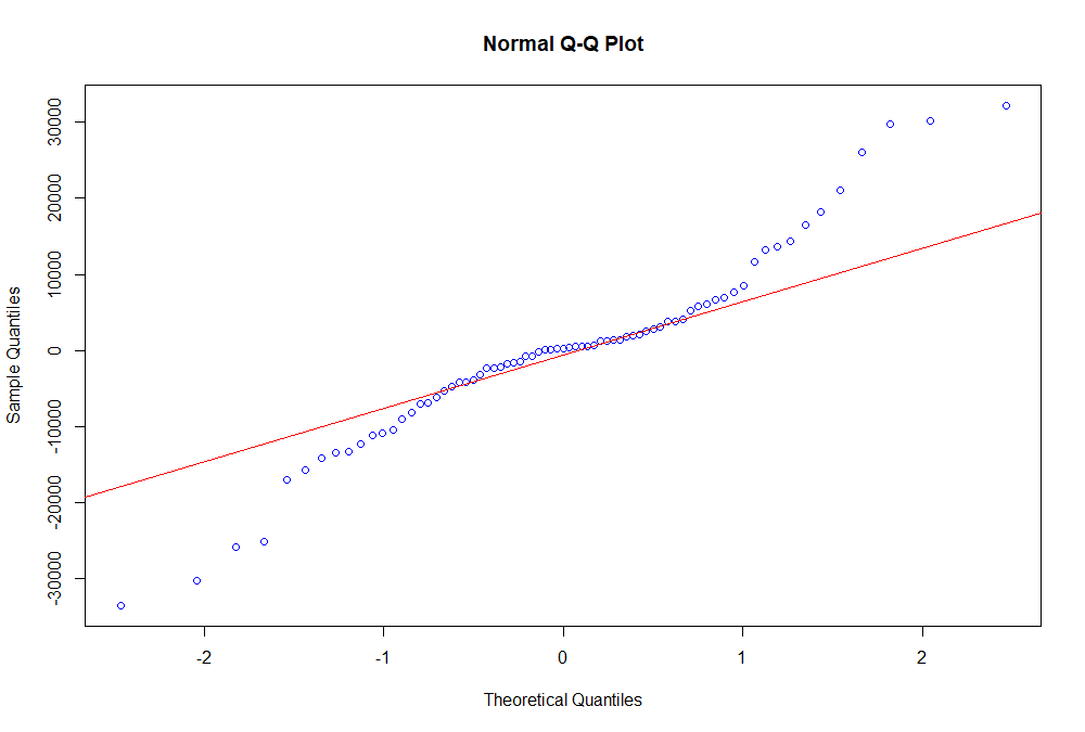
Source: compiled by the authors.
Figure 2. OLS Regression Plot - Total Sample
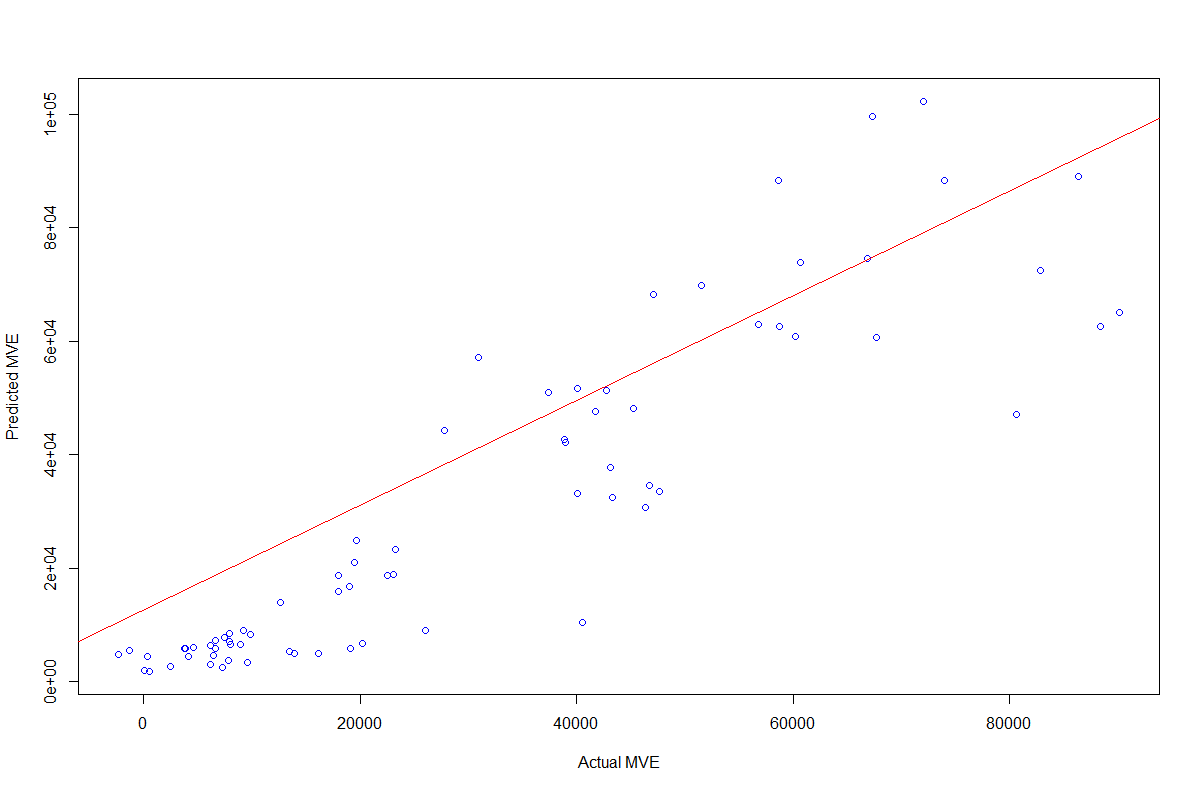
Source: compiled by the authors.
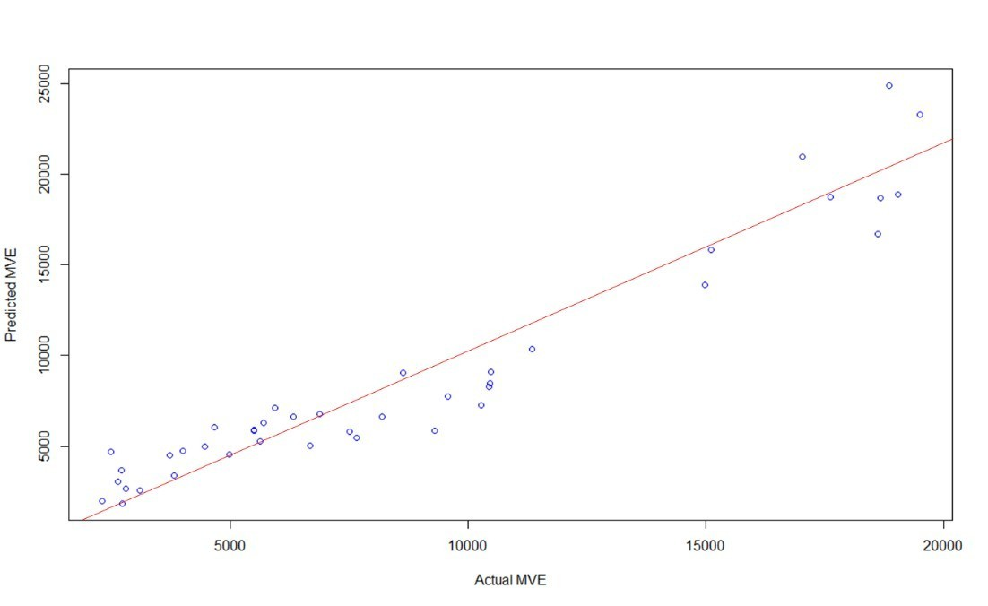
It can also be noted that the relationship between predicted values and real data for MVE presents different behaviors in the tranche corresponding to Santander and BBVA, as shown in Figure 3.
Figure 3. Actual MVE vs. Predicted MVE - Total Sample
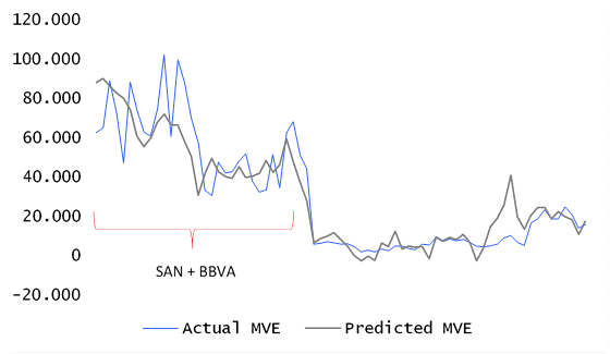
Source: compiled by the authors.
It may be argued that this result (the different behaviors in the tranche corresponding to Santander and BBVA) could be caused by a structural change in risk exposure. This is logical since both Santander and BBVA are global systemic banks, whose market values can be affected by many more variables that those included in our model which have been taken from financial statements only (for example: general economic status; evolution of economic indicators; evolution of values of other entities, etc.). This has been corroborated by running the Chow test (with a value of 7.25) in order to verify that the coefficients change substantially in the case of Santander and BBVA as compared to other entities.
The following tables (Table 6 and Table 7) include the statistics outcome for two separate regressions: one for a sample including all the entities except Santander and BBVA, and the other for a sample including only Santander and BBVA.
Table 6. OLS Regression analysis – Total Sample without Santander and BBVA
| Estimated coefficient | Std. Error | |
|---|---|---|
| BVAL | 6.58e+02 (6.826) *** | 9.64e+01 |
| REVA | 1.90e+02 (1.688) | 1.13e+02 |
| NONPERF | 2.08e+07 (2.308) * | 8.99e+06 |
| COREDEP | -5.70e+06 (-2.935) ** | 1.94e+06 |
| ROA | 7.89e+08 (6.122) *** | 1.29e+08 |
| Adjusted R-squared: 0.9708 | ||
| F-statistic: 273.2 | ||
| n = 41 | ||
| Note: significance codes are 0 ‘***’ 0.001 ‘**’ 0.01 ‘*’ 0.05 ‘.’ | ||
| t-value is included in brackets next to the estimated coefficient | ||
Source: compiled by the authors.
Table 7. OLS Regression analysis – Santander and BBVA
| Estimated coefficient | Std. Error | |
|---|---|---|
| BVAL | 7.26e+02 (4.882) *** | 1.49e+02 |
| REVA | -4.01e+02 (-0.654) | 6.14e+02 |
| NONPERF | 1.96e+08 (0.591) | 3.31e+08 |
| COREDEP | -3.49e+07 (-0.919) | 3.80e+07 |
| ROA | 5.62e+09 (3.394) ** | 1.66e+09 |
| Adjusted R-squared: 0.933 | ||
| F-statistic: 90.15 | ||
| n = 32 | ||
| Note: significance codes are 0 ‘***’ 0.001 ‘**’ 0.01 ‘*’ 0.05 ‘.’ | ||
| t-value is included in brackets next to the estimated coefficient | ||
Source: compiled by the authors.
As can be seen, the coefficients change dramatically, along with their significance. On the one hand, BVAL and ROA are the only significant variables for Santander and BBVA, whereas for the remainder of the entities, COREDEP and NONPERF are also significant. This means that the potential relationship between the MVAL of local entities19 and the information disclosed in their financial statements is much more substantial than in the case of global systemic banks.
The other relevant point to consider is that REVA is not relevant for either of the two data samples. This is an important conclusion of analysis. See further discussion in Section 6.
If we calibrate the model using the local entities (all the entities except Santander and BBVA), and eliminate REVA from the set of explanatory variables, it results in the statistics included in the table below (Table 8).
Table 8. OLS Regression analysis – Total Sample without Santander and BBVA and without REVA
| Estimated coefficient | Std. Error | |
|---|---|---|
| BVAL | 8.01e+02 (16.852) *** | 4.75e+01 |
| NONPERF | 2.35e+07 (2.592) * | 9.06e+06 |
| COREDEP | -6.08e+06 (-3.075) ** | 1.98e+06 |
| ROA | 7.65e+08 (5.825) *** | 1.31e+08 |
| Adjusted R-squared: 0.9693 | ||
| F-statistic: 324.6 | ||
| n = 41 | ||
| Note: significance codes are 0 ‘***’ 0.001 ‘**’ 0.01 ‘*’ 0.05 ‘.’ | ||
| t-value is included in brackets next to the estimated coefficient | ||
Source: compiled by the authors.
The results show that the explanatory power of these regressors is higher in terms of p-values, F-value, R2 and coefficient significance.
The figures below (Figure 4 and Figure 5) shows how the model performs as regards the MVAL data sample in terms of evolution and goodness of fit.
Figure 4. Actual MVE vs. Predicted MVE - Total Sample except Santander and BBVA
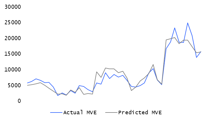
Source: compiled by the authors.
Figure 5. OLS goodness of fit plot - Total Sample except Santander and BBVA
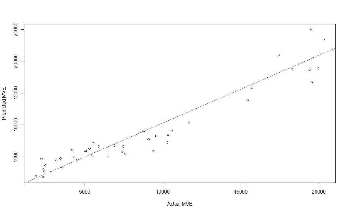
Source: compiled by the authors.
It should also be noted that no evidence of heteroskedasticity in the Breusch-Pagan test (assuming a constant linear relationship) was identified, and it is now possible to assume normality in residuals (see Figure 6).
Figure 6. Normal Q-Q Plot - Total Sample except Santander and BBVA
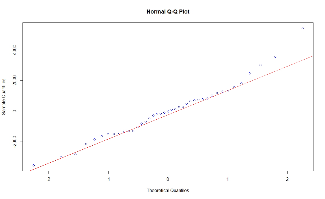
Source: compiled by the authors.
In addition, we verified that no outliers were identified among the sample, hence they all fall within the Cook distance lines: (see Figure 7)
Figure 7. Cook's distance Plot - Total Sample except Santander and BBVA
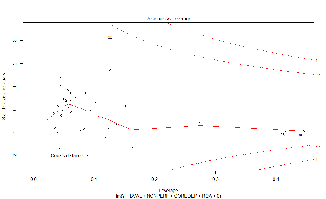
Source: compiled by the authors.
Furthermore, once the model was set with its explanatory variables, the relationship between said variables in terms of multicollinearity needed to be verified. This was done by analyzing the Variance Inflation Factor (VIF), computed for each pair of variables, and which resulted in the matrix shown in Table 9.
Table 9. VIF matrix – Total Sample without Santander and BBVA and without the REVA variable
| BVAL | NONPERF | COREDEP | ROA | |
|---|---|---|---|---|
| BVAL | - | 1.24 | 1.83 | 1.24 |
| NONPERF | 1.24 | - | 1.23 | 1.73 |
| COREDEP | 1.83 | 1.23 | - | 1.09 |
| ROA | 1.24 | 1.73 | 1.09 | - |
Source: compiled by the authors.
The outcome shows all VIFs below 2, hence it may be understood that no critical correlation exists between the variables.
Therefore, we conclude that (2) will be transformed into the following model:
\[\begin{equation} \label{eq4} \small \begin{split} \text{MVE}_{\text{ij}} =& \ BVAL_{\text{ij}}\beta_{\text{BVA}L_{\text{ij}}} + NONPERF_{\text{ij}}\beta_{\text{NONPER}F_{\text{ij}}}\\ & + \ COREDEP_{\text{ij}}\beta_{\text{COREDE}P_{\text{ij}}} + ROA_{\text{ij}}\beta_{\text{RO}A_{\text{ij}}} + \varepsilon \end{split} \ \ \ \ (4) \end{equation}\]
Furthermore, as indicated at the beginning of this Section, the use of panel data with OLS methods may lead to models being biased due to the existence of autocorrelation.
Due to the fact that the errors are unobservable in the linear model, particularly as regards panel data where relevant variables can be missed, the detection method should focus on the best available estimator, i.e. the residuals created in the regression. Therefore, we first performed the analysis by checking residual autocorrelation and partial autocorrelation plots (see Figure 8).
Figure 8. Residual autocorrelation and partial autocorrelation - Total Sample except Santander and BBVA
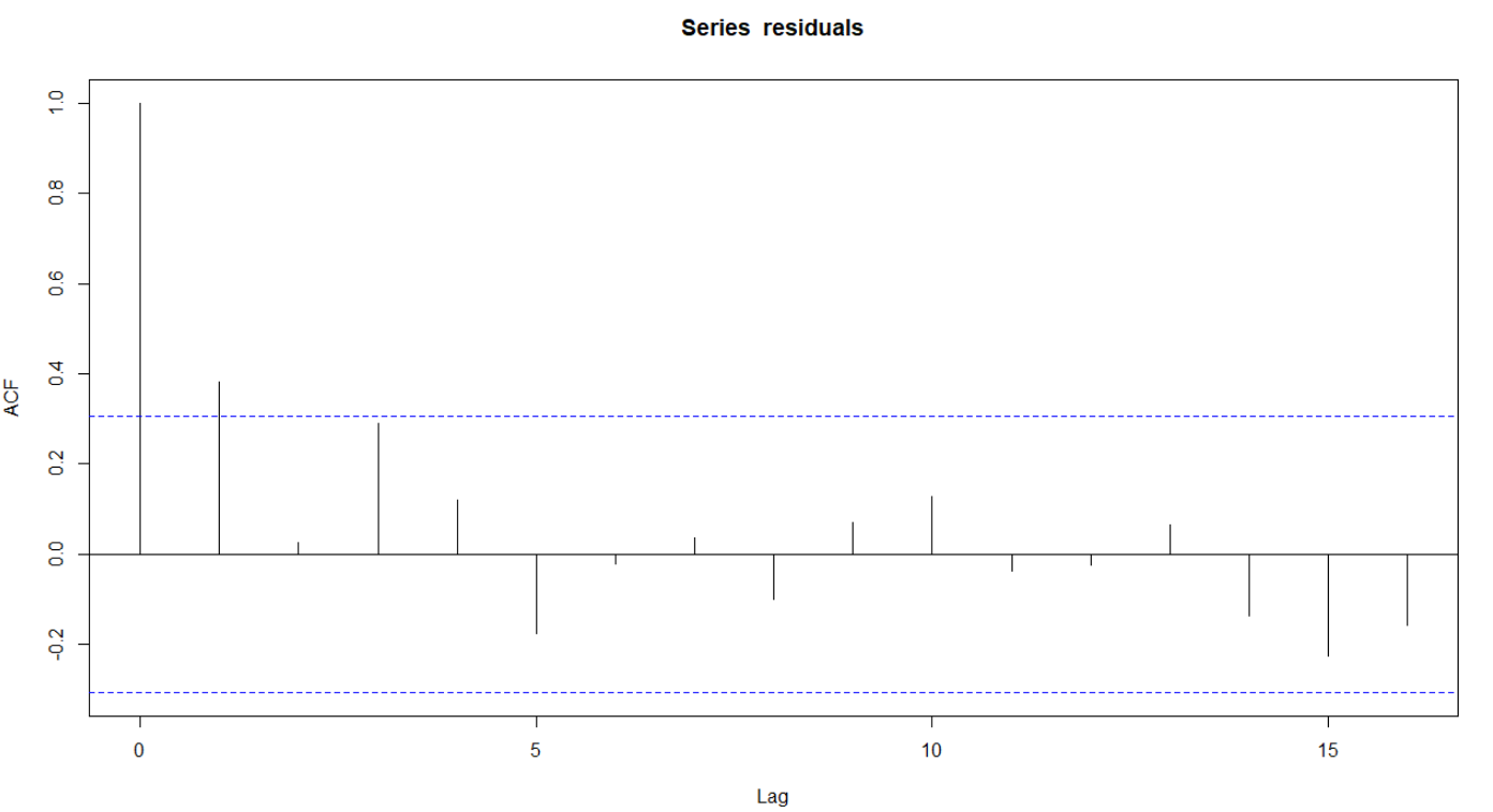
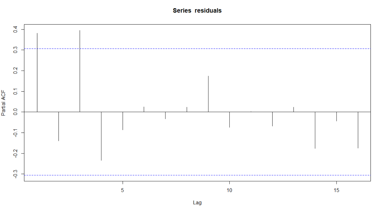
Source: compiled by the authors.
The dashed horizontal lines on the plots correspond to approximately 95% confidence limits. The general pattern of the autocorrelation and partial autocorrelation functions is suggestive of an autoregressive process of order 3 - AR(3) -.
Additionally, a Ljung-Box test (Ljung & Box, 1978) was performed in order to quantitatively analyze the weight of the autocorrelation for the given lags. Assuming the autoregressive process is of order 3, the statistic is 10.32, which is above that expected for a 95% confidence interval. This is another indicator of existing correlation in residuals.
5.3. Fixing autocorrelation via Generalized Least-Squares
It was found to be necessary to recalibrate the model (5) in order to include the autoregressive process, specifying the correlation structure to fit an AR(3). As indicated at the beginning of Section 5.2, the use of Generalized Least-Squares (GLS) can resolve this issue.
A GLS regression extends the Ordinary Least-Squares (OLS) estimation of the normal linear model by providing for possibly unequal error variances and for correlations between different errors. A common application of GLS estimation is to time-series regression, in which it is generally implausible to assume that errors are independent.
In the standard linear model, the OLS equation is:
\[\begin{equation} \label{eq5} \small y = \text{X}\beta + \varepsilon \ \ \ \ (5) \end{equation}\]
where \(y\) is the n x 1 response vector; \(X\) is an n x k +1 model matrix; \(\beta\) is a k + 1 x 1 vector of regression coefficients to estimate; and \(\varepsilon\) is an n x 1 vector of errors. Assuming that \(\varepsilon\ \sim\ N_{n}\left( 0,\ \ \sigma^{2}I_{n} \right),\) or at least that the errors are uncorrelated and equally variable, leads to the familiar OLS estimator of
\[\begin{equation} \label{eq6} \small b_{\text{OLS}} = \left( X^{'}X \right)^{- 1}X^{'}y \ \ \ \ (6) \end{equation}\]
with a covariance matrix
\[\begin{equation} \label{eq7} \small \text{Var}\left( b_{\text{OLS}} \right) = {\sigma^{2}\left( X^{'}X \right)}^{- 1} \ \ \ \ (7) \end{equation}\]
In the case of correlated errors, the GLS estimator is as follows,
\[\begin{equation} \label{eq8} \small b_{\text{GLS}} = \left( X^{'}\Sigma^{- 1}X \right)^{- 1}X^{'}\Sigma^{- 1}y \ \ \ \ (8) \end{equation}\]
with a covariance matrix
\[\begin{equation} \label{eq9} \small \text{Var}\left( b_{\text{GLS}} \right){= \left( X^{'}\Sigma^{- 1}X \right)}^{- 1} \ \ \ \ (9) \end{equation}\]
In the real application, the error covariance matrix \(\Sigma\) is not known, but can be estimated from the data along with the regression coefficients if we specify a structure of autocorrelated errors AR(p).
Therefore, if we know which the last lag is where autocorrelation may exist, we can then specify it in a GLS calibration.
5.4. Final results
In this case, in line with the output shown in Figure 8, the GLS model was calibrated with a maximum-likelihood estimation and specifying an AR(3), with the following results:
Table 10. GLS Regression analysis – Total Sample without Santander and BBVA and without REVA
| Estimated coefficient | Std. Error | |
|---|---|---|
| BVAL | 7,00E-01 (11,037) *** | 0.07 |
| NONPERF | 2,73E+04 (3,180) *** | 8,58E+03 |
| COREDEP | -4,82E+03 (-2,1227) · | 2,27E+03 |
| ROA | 7,22E+05 (6.0113) *** | 1,20E+05 |
| Adjusted R-squared: 0.9703 | ||
| n = 41 | ||
| Note: significance codes are 0 ‘***’ 0.001 ‘**’ 0.01 ‘*’ 0.05 ‘.’ | ||
| t-value is included in brackets next to the estimated coefficient | ||
Source: compiled by the authors.
As can be seen in comparison with Table 9, putting into the model the autocorrelation structure modifies the expected significance and weight of the several variables used, avoiding misinterpretation of their significance due to the potential autocorrelation or heteroskedasticity within the model, highly common when dealing with panel data.
Then, the adjusted R2 is a bit higher but close to that obtained with OLS (>0.9), with less residual standard error (1837 for GLS vs. 1848 for OLS). The weight of coefficients has changed, due to the correlation structured specified in the GLS. Also, the t-values show that COREDEP is less significant but, in contrast, NONPERF has increased its significance.
Figure 9. GLS goodness of fit plot-- Total Sample except Santander and BBVA
Source: compiled by the authors.
Figure 10. Actual MVE vs. Predicted MVE with OLS and with GLS - Total Sample except Santander and BBVA
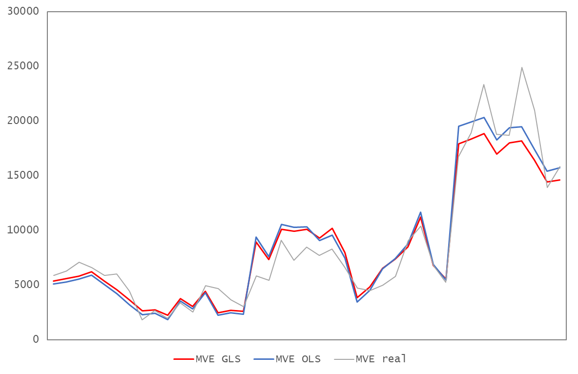
Source: compiled by the authors.
6. Results interpretation
According to the results described in Section 5, we may conclude that the first Hypothesis raised in Section 2 is not confirmed. Generally speaking, investors do not consider fair value disclosures in their investment decisions (at least as regards the sample entities). The REVA variable has no explanatory power in any of the regressions performed.
This result is different from the result obtained by other authors using other samples, even in Europe: Giner et al. (2020); Liao et al. (2020); Fiechter & Novotny-Farkas (2017); Siekkinen (2016); Drago et al. (2013); and Aurori et al. (2012). These authors find that investors do consider fair value disclosures in their investment decision.
Nevertheless, the result is coherent with the findings of several authors in relation to the lower fair value relevance in countries with strong enforcement (Liao et al., 2020). In this sense, and from a theoretical perspective, the difference setting in relation to other studies (the fact that our sample is only composed by Spanish entities) may influence the results. As we anticipated in Section 2.1 the political interference in financial reporting could lead to different results in our research in relation to other environments for several reasons:
A) The focus of the Central Bank supervision (and therefore the resources of the entity) is in other areas like the loan loss provisioning (as can be inferred from Giner & Mora, 2019 or Mora 2012). In this particular economy / jurisdiction, the supervision of the banking authority is specially focused on areas like the loan loss provisioning (as can be inferred from Giner & Mora, 2019 or Mora 2012) or the provisions related to the reposed assets (very significant in most of the years that compose the sample). This may make entities focus their resources to these areas and not to an area in which, initially, there is not a direct benefit for the bank. The low quality of this areas can make investors to have less confidence in this financial information.
B) The fact that financial statement users (investors) have less confidence on financial statements subject to political interference. For many authors, financial reporting (and accounting standards) can lose credibility and reliability if they are open to political intervention (Fogarty et al., 1994, Königsgruber, 2013).
On the other hand, from a more practical perspective, several different explanations may underlie our result. Firstly, it may be argued that entities do not assign the same resources to the fair value estimations of elements measured at fair value on the balance sheet as they do to fair value estimations of elements whose fair value is only disclosed (and with no equity effect). Therefore, the quality of disclosed fair value estimations would be rather low (or at least is perceived to be low by investors). Very few authors have previously put forward or analyzed this theory (see, as one of the few examples, Wilson 2001). Moreover, the problem is further compounded by the fact that many of the fair value estimations of elements whose fair value is only disclosed are Level 3 (for example, the loans portfolio given to retail customers).
The above argument can easily be corroborated by the explanations provided by the entities as regards fair value estimation. By way of example, Banco Popular states (in relation to its 2013 financial statements): “assets and liabilities that are measured at amortized cost in the balance sheet have been valued though future cash flow discounting using a risk-free curve without spread (zero coupon). This curve is generated from the quoted rates of the Spanish Public Debt that allows generating pure discount factors to calculate present values that the market admits as unbiased rates.”
This means that this entity is not correctly estimating the fair value of the amortized cost of assets and liabilities due to the fact that credit risk is not being taken into consideration (see paragraphs 34 along with B13, B16 and B17 of IFRS 13). The entity is assuming that the credit risk of financial assets (loans given to customer) and liabilities (deposits from customers and other debt instruments) can be assimilated to Spanish sovereign risk. This cannot be backed by historical facts: Banco Popular went bankrupt in 2017.
The following table (Table 11) shows the differences between the credit quality of Banco Popular and the Kingdom of Spain as at July 2014:
Table 11. Credit risk of Banco Popular vs. Kingdom of Spain (July 2014)
| Rating (S&P’s) | 5y Probability of Default (obtained from CDS quotes) | 10y Probability of Default (obtained from CDS quotes) | |
|---|---|---|---|
| Banco Popular | B+ | 15% | 32% |
| Kingdom of Spain | BBB | 6% | 19% |
Source: compiled by the authors using Reuters.
A further example is provided by Renta 4, who states (for all the years included in the sample) that there is no material difference between the book value and the fair value of financial assets and liabilities measured at amortized cost. Similarly, Sabadell put forward the same argument for the years 2004 to 2008 (while this bank maintained a significant loan portfolio).
The second explanation for this result (i.e. the first Hypothesis not being confirmed) is related to the level at which fair values are classified by the entities. According to the findings of previous authors, Level 3 valuations are less relevant than those at Levels 1 and 2 (Kolev, 2019; Goh et al., 2015; Bosch, 2012; Song et al., 2010). In our sample, a significant percentage of fair values are classified as Level 3. In the case of assets, the majority of elements consists of loans given to retail customers (Level 3). With regards to liabilities, the majority of elements consists of current accounts which for many banks are Level 3 due to a non-observable input, i.e. the portfolio payment structure.
Other explanations may be as follows:
The timeframe included in the sample represents a period of time during which the entities in the sample faced several important problems. Initially new IFRS standards came into effect (with no previous experience as to their application). Subsequently, the financial crisis began in 2008, and finally, benchmark interest rates became extremely low (even negative in some cases). This may have led to the entities utilize their resources to solve these problems and not to estimate the disclosed fair values.
The Bank of Spain (and nowadays the European Central Bank also) could demonstrate a higher level of concern for stability and balance sheet issues (including, for example, loan loss provisioning) than for informative disclosures.
One additional general conclusion arising from our research is that, in the case of global systemic banks (Santander and BBVA), the MVE factor cannot be seen as highly related to the information disclosed in financial statements on a consistent basis. The MVE for banks such as these may be affected by other factors such as events occurring in financial markets; general economic indicators, etc. This is logical since the return, particularly in this type of bank, can be seen as a determinant metric of general financial stability (due to it is direct correlation with the level of interest rates in the markets).
In this sense, local credit institutions (all the entities included in the sample except Santander and BBVA) may be more dependent on metrics disclosed in the financial statements, particularly regarding the structural risk provided by core deposits or the proportion of non-performing assets.
As regards the second Hypothesis, it was found that all three of the ratios used (NONPERF, COREDEP and ROA) have explanatory power on the MVA for local credit institutions but not for Santander and BBVA (in the case of the latter, only ROA is significant).
Generally, recent authors have not used goodwill ratios (except for Barth et al., 1996, and Brickner, 2003) therefore we cannot compare our results with those of other authors. In relation to Brickner (2003), using a sample of 867 calendar year-end banks during the period of 1996 and 1997 he finds both “non-performing loans” ratio (NONPERF) and “core deposits ratio” (COREDEP) as significant (as in our case for local credit institutions).
7. Concluding remarks
We analyze the incremental value relevance of financial instruments fair value over historical cost. We use a sample that includes Spanish quoted credit institutions, and we apply an Ohlson model. The period covered goes from 2004 to 2019.
As developed in Section 2.1, our research implies a relevant new perspective in value relevance literature due to the sample used and the time frame applied. Currently, no research exists which applies the "Ohlson Model" to a sample only including Spanish quoted credit institutions. This specific setting is different from others as evidence of political interference does exist in financial reporting within Spain’s financial industry (Giner & Mora, 2019 and 2020). In fact, Spain is a unique case in Europe and other developed economies in which the Central Bank issues accounting standards and directly supervises the application of those standards. For Burgstahler et al. (2006), since a country’s institutional factors define and shape firms’ financial reporting incentives, they play an integral role in determining the properties of accounting numbers.
Our results show that fair value disclosures are not relevant for equity investors i.e. these investors do not consider this information in their investment decisions.
This result, which is different from most findings from previous works, is likely to be influenced by the specific characteristics of Spanish credit institutions and its regulation framework. In previous Section we also discuss other potential, more direct explanations for our result, evidenced by the analysis of the financial statements of the entities.
Our work contributes to the current debate in relation to the application of fair value as a measurement model for more elements in the balance sheet (specially in financial instruments area). It seems that, in the case of Spanish credit entities, greater resources should be assigned to the estimations behind fair value disclosures of financial instruments not measured at fair value in the balance sheet. The objective of this effort should be providing higher quality revaluation estimates so that investors can rely on this information. This could be even a first step prior to including this information in the balance sheet (in relation to current IASB and FASB fair value debate).
This is particularly important as, in other European and international contexts, previous research shows that fair value disclosures are value-relevant and this could be a disadvantage for Spanish banks.
The limitations of our research are related to the sample size (which cannot be bigger as we have included all quoted Spanish credit entities and we have used financial statements from the first year in which they started to apply IFRS onwards). Moreover, we had to split our sample into two parts as there are two banks (Santander and BBVA) with a different behavior in comparison to the remaining entities in the sample. These two entities are global systemic banks and their quoted price is influenced by other global factors.