Common distress and reorganization patterns by sector and country for SMEs in six European countries using PDFR

ABSTRACT

This study contributes to identifying common distress patterns in financial indicators by sector and country in Finland, France, Germany, Italy, Portugal, and Spain as well as ex-post signals of reorganization success. We use PDFR that provides a distance-to-failure measure and allows us to track the behavior of different features of the firm proxied by accounting ratios. Our results show that indicators of financial structure, followed by working capital, profitability on assets, margin over sales and cash flow to assets, are the most discriminant variables of failed SMEs across all sectors and countries analyzed. By contrast, during reorganization, return on assets and its components are the main initial drivers of recovery, whereas the financial structure factors show a progressive but slow recovery. Boosting and Z-scores are used for robustness.

Patrones comunes de fracaso y reorganización por sector y país para las PYMEs de seis países europeos utilizando PDFR

RESUMEN

Este estudio contribuye a la identificación de patrones comunes de fracaso en indicadores financieros por sector y país en Alemania, España, Finlandia, Francia, Italia y Portugal, así como a la identificación de patrones comunes de éxito en la reorganización. Utilizamos PDFR, que proporciona una medida de distancia al fracaso y permite hacer un seguimiento de la evolución de la empresa a través de sus ratios contables. Nuestros resultados muestran que los indicadores de estructura financiera, seguidos de fondo de maniobra, rentabilidad sobre activos, margen sobre ventas y *cashflow* sobre activos, son las variables más discriminantes de las pymes clasificadas como fracasadas, en todos los sectores y países analizados. En contraste, durante la reorganización, la rentabilidad sobre activos y sus componentes son los principales inductores iniciales de la recuperación, mientras que los indicadores de estructura financiera muestran una progresiva pero lenta recuperación. Se utilizan Boosting y Z-score como medidas de robustez.

1. Introduction

It is generally accepted that there are multiple reasons behind business failure. The problems may appear from the creation, after growing to a level that the managers cannot cope with, after several years of gradual decline, or suddenly as a result of external shocks (Argenti, 1976). The factors of business deterioration may be related to the owners' or the managers' characteristics, the firms' resources and functioning, and environmental conditions (Keasey & Watson, 1991; Mayr et al., 2017). Consequently, symptoms and duration of the failure process vary remarkably (Lukason & Laitinen, 2019).

In the case of SMEs, the range of possibilities is especially wide. Firms failing in a short period after opening and firms finding problems to change dimension are mostly SMEs. The influence of owners' and managers' characteristics is logically higher when their number is small, the SMEs' access to resources is more limited (Geroski et al., 2010; Headd, 2003), and SMEs are more vulnerable to environmental pressures (Box, 2008). The reasons include reduced diversification, lack of scale effects, and smaller risk buffers (Aldrich & Auster, 1986; Geroski et al., 2010) jointly with increased dependence on specific stakeholders (Herbane, 2012).

Business reorganization has not reached the level of advanced research. In fact, empirical literature on the factors behind business reorganization remains scarce and inconclusive. The purpose of reorganizing instead of liquidating a firm is to restructure financing to maintain concern and employment while generating return for the owners. Thus, when the business could be profitable but temporary factors have created a bad situation, reorganization is more efficient than liquidation.

Looking ahead, SMEs' reorganization will depend not only on access to financial (Gutiérrez-Urtiaga, 2000) and economic resources but also on the managerial competence and ability to implement the necessary changes (Westhead et al., 2001). In the long run, reorganization requires that the company successfully overcomes the causes of its problems to regain its credit-worthiness and its competitive market position (Mayr et al., 2017). Basically, after learning from failure, the firm should become profitable in a sustainable basis. Furthermore, in case the company is involved in a legal reorganization process (under bankruptcy codes), it must fulfill the specific requirements of the country (Claessens & Klapper, 2005; La Porta et al., 1998).

The objective of this paper is to analyze how SMEs reorganize to recover after inclusion in the group of failed or close-to-fail firms. This objective concerns the behavior of financial indicators to find out the starting point of the variables traditionally found as discriminant to identify failed firms, that is, how far they are from the benchmarks by year, country, and sector; and the evolution during the subsequent process of recovery, that is, what financial indicators are contributing to that recovery, how much and when do they approximate to the benchmarks. Our study avoids the influence of uncontrollable environmental conditions by eliminating the year, country, and sector biases by comparing with benchmarks to focus mainly on firm's performance differences.

Our interest is checking the behavior of financial indicators during successful reorganization to check if the basic forces behind failure and reorganization are relatively stable across time, countries, and sectors in line with the results found by Lev (1969) and Platt & Platt (1990; 1991) when the sector bias was eliminated.

In the context of bankrupt SMEs, there are some works concerned for the evolution of financial ratios (Laitinen, 2018) and the identification of risk profiles (Koyuncugil & Ozgulbas, 2012), however, there are no previous research analyses performed for firms under reorganization to examine the evolution of financial indicators in respect of appropriate benchmarks that account for the year, country, and sector environments. Therefore, our study is of interest for analysts, researchers and academics concerned in assessing the firm's financial performance taking into account the effect (or the lack of effect) of the environment in terms of year, country, and sector. In the context of firms close-to-failure and reorganization, our results are of interest for investors, creditors, regulators, and the public administration as stakeholders putting their money (and work) at risk when their assessment of the firm's recovery ability is wrong.

We apply the PDFR methodology (Tascón et al., 2018) to obtain distance-to-failure scores of all the SMEs in six European countries (Finland, France, Germany, Italy, Portugal, and Spain) and four sectors (manufacturing, construction, business services and trade) during the period 2010-2016. This methodology is based on statistical measures, specifically the percentile differences of accounting ratios between the group of failed firms and the population to which that group belongs.

Using PDFR, we identify the factors that have acted as drivers for firms to enter in distress and what factors have contributed to help firms to recover. This study is performed by sector and year inside each country under analysis. Our final sample includes 2,453,508 European firm-year data, of which 240,595 failed according to the criterion applied in this study. For comparison purposes, the Boosting model was used to identify the accounting ratios proxying for features behind failure and reorganization. Boosting is a machine learning methodology of recent application in the research line on failure (Sun et al., 2014; Verikas et al., 2010). Furthermore, we have computed the well-known Z-scores of the firms under reorganization in our analysis and compare the results with those of the scores obtained by the PDFR methodology.

Our main contribution is a description of the evolution of successful reorganized firms in terms of the individual financial indicators with a demonstrated role in the process, in a wide study of European SMEs. This type of by-factor analysis not previously made in the literature has allowed us to identify a common pattern across countries and sectors, concerning the factors behind failure and reorganization of SMEs in the six European countries and four sectors analyzed. The most discriminant factors for failed firms referred to financial structure, followed by a group of five ratios representing the following factors: working capital, return on assets, sales margin, and cash flow generation. By contrast, return on assets followed by sales margin and cash flow are the most discriminant factors during the first year of reorganization. Financial and economic structures show progressive but slow recovery such that three years is an insufficient period to recover to the central levels of the population. In addition, we quantify the distance to failure and simultaneously the distance to recovery using scores. The scores indicate how difficult it is for firms in a failure situation to recover to the central levels of the population.

The paper is structured as follows. Section two gathers some aspects of previous evidence on business reorganization after failure, especially oriented to the behavior of financial indicators in SMEs. This section also gathers the findings of previous literature on the effect of time, country, and sector elements over financial indicator benchmarks. Section three describes the sample and explains methodological aspects. Section four displays our results on variable relevance as well as scores and distances to failure during reorganization. Section five concludes.

2. Literature review on reorganization in SMEs

2.1. Factors behind SMEs' reorganization

This paper deals with the evolution of financial indicators during business reorganization of SMEs. Business reorganization represents a research stream within business failure that originated more recently. It shows a still incipient development not only in Europe, but also in the general international arena.

Our concern is the perspective of the survivor firms, namely, how and why they get to recover after being included in the group of failed firms. In this field, studies before 2000 are very scarce. Thus, Campbell (1996) identifies factors, such as size, asset profitability, the number of secured creditors, the presence of unencumbered assets, and the number of undersecured secured creditors, in an empirical study applied to closely held firms. Pandit et al. (2000) study financially troubled small firms in the United Kingdom and find that the process is generally successful when the economic fundamentals of the business are sound regardless of the firm's line of activity. Gutiérrez-Urtiaga (2000) finds that access to short-term liabilities positively affect sales and net income of SMEs during crisis periods, thus favouring a subsequent reorganization.

From that point, the regulation about the conditions for failed firms that are included in reorganization processes has attracted the attention of research in many countries. Most studies concern US firms. Denis & Rodgers (2007) find that firms are more likely to achieve positive post reorganization profitability when they have significantly reduced assets and liabilities during the process. Altman et al. (2009) use a modified version of the well-known Altmant's Z-score to assess the health of industrial companies as they emerge from Ch.11 and survive as well as those that later file again. The authors find that firms filing for a second time had significantly higher leverage and lower profitability shortly after emerging the first time. Altman explores the role played by the debt market and the hedge funds in the bankruptcy-reorganization process of US firms (Altman 2014b).

Other studies have contributed to this research in several European countries. For example, in Belgium, Dewaelheyns & Van Hulle (2008) show that bankruptcy code reform reduces the small and micro business bankruptcy rates, but the effect is only significant in certain industries (manufacturing and trade).

In the United Kingdom, Cook et al. (2012) propose a resource-based approach to assess the viability of failed SMEs. According to this approach, a firm with strong resources pushed into failure by temporary factors is more likely to succeed in the reorganization.

In Italy, Rodano et al. (2016) study the bankruptcy law reforms and find that the 2005 reorganization procedures facilitate loan renegotiations, whereas the 2006 reform strengthens creditor rights in liquidation.

In Spain, Segovia & Camacho (2012) use artificial intelligence methodologies to identify the indicators of possible success in reorganization and find that those factors include sector, size, taking part of a group, and return on assets. Later, Camacho et al. (2015) apply this type of methodology to the SMEs' reorganization and demonstrate that their model could reduce delays and costs in choosing between reorganization and liquidation using only five variables (sector, size, number of shareholdings, return on assets, and cash ratio).

In Finland, Laitinen (2011) uses logistic regression analysis with financial and nonfinancial information to conclude that a greater portion of firms that filed for reorganization under the Finnish Bankruptcy Act are nonviable, whereas many firms classified as bankrupt are viable. In a previous study, Laitinen (2008) finds that the information provided by the firms to enter the reorganization plan can improve the quality of the model, but the accuracy of the classification is not significantly better.

To date, the studies focused on regulation have analyzed whether firms should be reorganized or not based on possibilities of success (Altman et al., 2009; Camacho et al., 2015; Cook et al., 2012; Denis & Rodgers, 2007; Laitinen, 2011; Segovia & Camacho, 2012), but our first objective goes a step beyond towards the orientation of the reorganization by sector and by country, paying attention to the evolution of the individual financial indicators.

The most recent studies in this field of research address how firms reorganized and recovered after the global financial crisis started in 2007-2008. Kelly et al. (2015) find that during the crisis, the survival of Irish small firms mostly depended on banking credit. For Mayr et al. (2017), the pivotal factor in the turnaround of Austrian SMEs is repositioning, which is characterized by a unique selling proposition, innovation, change, and integration into networks. Cowling et al. (2018) analyze the firm's age and the entrepreneur's experience with respect to the SMEs performance after the crisis. They find the firm's age is related to growth, whereas the entrepreneurial experience seems to have little value in a unique and uncertain environment. Van Hoang et al. (2018) study how the crisis has affected the capital structure of French microfirms and find that firms survive by relying mostly on internal sources of financing. In sum, changes in indebtedness seem relevant for reorganization processes to recover from a crisis period.

Concerning the identification of determining factors for the reorganization of distressed firms, the initial studies previously mentioned (Campbell, 1996; Pandit et al., 2000) note the soundness of the business as reflected in factors, such as size, return on assets and several elements of indebtedness. Similarly, in France, Ayadi et al. (2020) identify size, profitability, liquidity, and leverage as firm-specific factors to accelerate or reduce the time to failure of reorganized firms, as well as an industry factor (industry profitability) and two macroeconomic factors (inflation rate and variation of short-term interest rates). Analyzing small entrepreneurial firms, Laitinen (2014) demonstrates that the management accounting change does not improve reorganization. According to their activity, Altman (2014a) finds different survivor profiles in the reorganization stage, and Dewaelheyns & Van Hulle (2008) show that the Belgian bankruptcy code produced different by-sector effects. Therefore, it can be derived that the financial indicators converge around the same factors identified as discriminant in case of failure, as expected, although previous research has not paid attention to the individual contribution of each factor and the evolution during the recovery. Concerning the role of the sector and country environments, the evidence is scarce and a more in-depth analysis is needed.

In this study, we perform a cross-country and by-sector analysis of failure and reorganization of SMEs after their proximity to failure. Our focus is the relative relevance of the different accounting ratios taken as proxies of economic and financial features of the firm.

2.2. Changing benchmarks by year, country, and sector

Analyzing how healthy a firm is requires a benchmark to compare against. The same can be said concerning how close-to-failure it is and how far from failure the firm can be after a reorganization process. The literature offers numerous evidence and signs of evolution in performance benchmarks over time¹, as well as differences of those performance benchmarks between countries and across sectors (Liou & Smith, 2007; Mensah, 1984; Platt & Platt, 1990). Modelling accuracy deteriorates with those changes of benchmarks, introducing noise and biasing the score, assessment, or qualification attributed by the specific model used and hindering the diagnosis and the subsequent reorganization measures to be applied.

For example, a problem identified in the process of predicting business failure is that ex post conditions during the model validation (and later application) vary in respect to ex ante conditions in which the models were calibrated (Platt & Platt, 1990).

The evolution of benchmarks due to data instability over time may be attributed to macroeconomic forces with effect on the business environment, such as changes in inflation rates, interest rates, employment rates, credit availability and other factors of monetary policy (Liou & Smith, 2007; Mensah, 1984). The economic cycle is a determinant factor (Mensah, 1984) as periods of economic recession directly make business, liquidity, and profitability to decline (Habib et al., 2020).

Ayadi et al. (2020) find that inflation has a positive effect but the variation of short-term interest rates has a negative effect on the survival of reorganized firms in France. In the same line, Hazak & Männasoo (2010) find that higher real interest rates trigger bankruptcy whereas a credit crunch and real exchange rate appreciations hamper the firm's survival. Also, in the UK, Bhattacharjee et al. (2009a) find freshly listed firms more likely to go bankrupt during unstable periods with sharp increases of inflation and sharp depreciation of the currency.

Other country-specific factors with effect on the variation of benchmarks from one year to another are changes in regulation, in special that on bankruptcy (López-Gutiérrez et al., 2012; Rico & Puig, 2019). Thus, firms' reorganization under the US bankrupcy law (Chapter 11) induces different response to macroeconomic instability in terms of bankruptcy than that in the UK, because the US regulation temporarily protects distressed firms from bankruptcy (Bhattacharjee et al., 2009b). Notwithstanding, Liu (2004) finds that the UK Insolvency Act has a mitigating effect on company liquidations. It happens not only in UK, but also in Germany and Spain, where López-Gutiérrez et al. (2012) find that bankruptcy laws have favored the firm's continuity at the expense of reducing protection for creditors.

In addition to the previous macroeconomic factors inducing differences in the evolution of the benchmarks, legal, cultural, and regulatory systems are to a great extent country-specific (Liou & Smith, 2007) pointing to the necessity for country-specific benchmarks. For example, Hazak & Männasoo (2010) evidence that old and new EU member states suffer the effect of macroeconomic factors (interest and exchange rates) in a different way; and Makropoulos et al. (2020b) find that by-country economic environment and legal tradition affect the transition from failure to liquidation of European SMEs.

Literature about the effect of macroeconomic factors on firms' behavior not only has paid attention to bankruptcy and survival, but there are also empirical evidence of the effect of macroeconomic elements on some of the most salient financial indicators of business failure and reorganization, such as financing and profitability. Here we gather some references specifically referred to European SMEs.

Financing of European SMEs is chosen (Andrieu et al., 2018) and show patterns in line with country-specific differences coming from macroeconomic factors such as inflation rates and volatilities, GDP per capita, and unemployment rates (Masiak et al., 2017). The reasons behind differences in the European economic environment by country can be (Demirgüç-Kunt & Maksimovic 2001): the quality of the legal system, and the concentration of the banking sector. Using data from 40 countries, Demirgüç-Kunt & Maksimovic (2002) find that the development of the legal system is determinant for the access to external finance, inducing differences in firm's growth rates. Furthermore, some financing tools, such as trade credit, have been evidenced to improve the likelihood of European SMEs' survival during the post-crisis years (McGuinness et al., 2018). Specifically, in UK, Makropoulos et al. (2020a) find that all different failure processes identified in their sample of SMEs are affected by credit availability.

Profitability of European SMEs is found by Gaganis et al. (2019) to be shaped by country-specific factors as well. These authors evidence that profitability is favored by the lack of corruption, easier conditions to obtain credit, fewer regulation on business entering, operating, and exit, as well as by some dimensions of country-specific culture, political stability and institutional development.

However, industrial cycles, addressed by technological obsolescence, sociological and demographical changes, and changing fashion (Harrigan, 1980), can remarkably differ from economic cycles. This is the reason for the necessity of industry benchmarks. In fact, the greater the specialization of the items included in the ratios or variables analyzed, the greater the incidence of the economic characteristics of the industries in the analysis results (Gupta & Huefner, 1972; McLeay & Fieldsend, 1987). Thus, financial indicators with a relevant role in failure and reorganization like cost/revenue and capital structure show patterns that use to be industry-specific (Lev, 1969; Liou & Smith, 2007), being industry an important determinant of retrenchment success (Guthrie & Datta, 2008). Consequently, a wide number of failure analyses have been performed on a sample of a unique industry, such as the construction industry (Abidali & Harris, 1995; Acosta-González et al., 2019; Alaka et al., 2016; Horta & Camanho, 2013; Sueyoshi & Goto, 2009; Tascón et al., 2018) to mention only one.

Industry-specific factors have also been analyzed as drivers of the most salient financial indicators of business failure and reorganization, that are financing and profitability. Thus, the manufacturing industry is more likely to obtain external financing than other industries due to the value attributed to the productive assets as collateral (Andrieu et al., 2018). As for profitability, Bamiatzi et al. (2016) results support the importance of industry-specific factors, suggesting that industry structure -market concentration, competition intensity, and entry barriers- and cycles - industry maturity- affect the firm's ability to become profitable.

Finally, the three elements mentioned behind the changing benchmarks for financial indicators -year, country, and industry- combine each other as some authors have brought to light. This way, the industry growth patterns vary between countries due to economic and financial development. Chang & Dasgupta (2002) find that in countries with closer GDP per capita, industrial growth shows similar patterns. Also, industries with superior financial needs can grow faster in countries with more developed financial markets (Beck & Levine, 2002; Chang & Dasgupta, 2002; Rajan & Zingales, 1998); and when the legal system is investor protective, industries' growth is boosted (Beck & Levine, 2002). According to Bamiatzi et al. (2016), in recessionary periods industry and country effects are weaker and firm effects stronger, especially for countries in emerging economies. Goddard et al. (2009) evidence that country and industry factors originate differences in profitability and growth of manufacturing industries in European countries.

In the case of SMEs, Clark et al. (2004) argue that internal resources are rarely enough to make business in European and global markets. That is the reason why country and industry factors seem to address to a greater extent SMEs' competitive strategies.

To overcome the problem of changing benchmarks in the three dimensions (time, country, and industry) the solutions used by researchers are varied (Liou & Smith, 2007; Khoja et al., 2019; Rico & Puig, 2019). (1) The analysis can be performed for a unique industry, being the usual that only one country and one year were taken for the study. (2) Paired-matching samples by industry have been used, being again the usual that the study was made for one country during a single period or by-period. (3) In parametric methodologies, such as regressions, control variables for industry, country, and period can be included. (4) By-industry mean or median values of the financial indicators can be compared with by-firm values of those indicators, usually by country and year. (5) Financial indicators can be standardized by using the industry median, usually by country and year. (6) Industry 'norms' can be stablished and financial indicators can be positioned within a certain industry's distribution for each financial indicator, usually by country and year.

The objective of the study conditions the alternative way of coping with these three causes of changing benchmarks. When the aim of the study is the classification of firms between the groups of 'healthy' or 'close-to failure' firms, solutions (1), (2), (3) and (5) are effective. (1) and (2) compare firms from homogeneous groups (same year, country, and industry); (3) adds controls for the three elements, thus isolating the effect of other financial indicators on the classification; and (5) divides firm's values by the central value of the group taken as benchmark, that should be computed by industry, country, and year and this way compares values free from differences coming from those environments. When the objective of the study is to stablish a benchmark not biased by the year, country, and industry, in order to know if the financial indicators of a firm are outliers and if they are better or worse than those of the group of comparison (Liou & Smith, 2007), alternatives (4) and (6) are more appropriate.

In the case of the current study, to identify the relevant actors of successful reorganization among the financial indicators, with independence of the destabilizing environment (year, country, and industry) in which this recovery takes place, options (4) and (6) could be good. The selected methodology, PDFR, uses both instruments: central values by industry, country, and year to be compared with the values obtained by individual firms for each financial indicator; and a distribution for each financial indicator in which the 'norm' of the population and the values for individual firms are positioned.

Considering the vast previous empirical literature on failure analysis and the more recent and incomplete evidence found in the research stream of reorganization, concerning the financial indicators with a discriminant role in the processes; and taking into account the vast empirical literature on the effect over benchmarks of the evolution of macroeconomic factors, the country-specific elements, and the sector-specific determinants, we hypothesize that all those elements of benchmark in stabilization must be neutralized to identify the financial indicators behind failure and reorganization. The sector should be a differential factor of the variable relevance, although the effect is expected to vary across countries, in line with the different pace of economic cycles by country. The country should not play such a relevant differential role considering that the six countries selected are placed in the same geographical area and are included in the European Union, a relevant factor of globalization both in the economic and the financial arenas for the six countries studied, even though the literature identifies resilient differences on legal, cultural, and regulatory systems among European countries.

3. Data and model implementation

3.1. Data and variables

The data used in our empirical analysis are extracted from Orbis, a database published by Bureau van Dijk (BvD). Our population under study is composed of SMEs in the six European countries with the highest number of SMEs: Finland, France, Germany, Italy, Portugal, and Spain. We have analyzed all SMEs in the four sectors selected in all the European countries where the number of those SMEs was enough to perform the reorganization analysis designed from 2010 to 2016 to obtain a reasonable representativeness of the statistical measures. All active, private and public limited companies with a maximum number of 250 employees, less than or equal to €50 million operating revenue, and less than or equal to €43 million in total assets² existing during the whole period 2009-2016 were selected from the database. To avoid bias from dependence (as shown by Beaver et al., 2018), we have selected those companies for which all shareholders or all shareholders with a stake greater than 25 percent are individuals or employees (according to the Orbis database).

Concerning the industry classification, we follow Dewaelheyns & Van Hulle (2008) and Harhoff et al. (1998) to apply a broad classification system in which only four major industry groups are identified: manufacturing, construction, trade and business services (excluding financials). Thus, the annual number of failed firms per industry group is sufficiently large to avoid erratic movements in the failure rate. We classify codes 10-32, 35, 58, 59 as manufacturing; 41-43 as construction; 33, 36-39, 452, 49-53, 55, 56, 60-63, 68-75, 77-82, 85-88, 90-96 as business services; 451, 453, 454, 46, 47 as trade. Therefore, we excluded from the by-sector study the primary sector and financial services (64-66) as well as 84 (public administration and defense: mandatory social security) and 97-99 codes (nonbusiness activities by households or organizations).

To analyze the failed group of firms inside the entire population, we create a failure firm-year indicator equal to one if the firm's equity is negative or zero and equal to zero when the firms' equity is positive. Thus, our computing of failure belongs to the concept of financial crisis as the firm's situation in which a company can no longer meet financial obligations and/or liabilities are greater than the company's assets (Mayr et al., 2017). In the current study, a main interest is the process of reorganization after a distress period; therefore, the official declaration is a secondary issue. In fact, bankrupt, dissolved and extinct firms are mostly beyond our group of interest due to their scarce possibilities to reorganize (Laitinen, 2011; Mayr et al., 2017).

Our general definition of failure based on patrimonial status avoids some problems of classification. Thus, firms that only declare bankruptcy for strategic reasons (Balcaen & Ooghe, 2006; Headd, 2003, Klobucnik et al., 2017) or, in the case of small firms, firms that dissolve or extinct for retirement, illness and other reasons affecting the continuity of the owners (Baixauli & Módica-Milo, 2010; Cochran, 1981) are not considered failed in our study. At the other extreme, firms with negative or null equity were considered as failed firms although they may remain active for years (Klobucnik et al., 2017). In fact, those firms showing early warning of financial distress confer large benefits to the firms' stakeholders (Keasey & Watson, 1991). From our point of view, those firms are the main objects of the reorganization study.

Considering the selected measure of failure based on the accounting value of the firm's equity, we expect a higher correlation of that measure with some related ratios, such as total liabilities to total assets, net income to total assets or reserves to total assets. However, our study is not interested in the prediction of failure but in the evolution of the most discriminant factors of failure during the later process of reorganization and, in this context, the accounting definition of failure/health starting from the value of equity is the most adequate for SMEs. Even if there is a necessary positive correlation between the negative equity and the firm's indebtedness, it is widely variable and does not represent an obstacle for performing the present analysis, just a limitation to be taken into account when results are interpreted. Both profitability and financial structure are critical factors to be analyzed during the reorganization process as they are critical for the firms' financial health which is represented by the accounting equity³.

Similar to the previous applications of the PDFR (Castaño, 2015; Tascón et al., 2018), our selection of variables is based on the literature on SME business failure. We select the most frequent financial ratios that are significant in identifying and predicting business failure,⁴ including Total Liabilities to Total Assets (TL/TA or R1), Current Assets to Current Liabilities (CA/CL or R2), Earnings Before Interests and Taxes to Total Assets (EBIT/TA or R3), Net Income to Total Assets (NI/TA or R4), Current Assets to Total Assets (CA/TA or R5), Financial Expenses to Total Liabilities (FE/TL or R6), Retained Earnings to Total Assets (RE/TA or R7), Cash Flow to Total Liabilities (CF/TL or R8), Net Income to Sales (NI/Sales or R9), and Sales to Total Assets (Sales/TA or R10). Considering our focus on the reorganization process, we have extended the model by adding Sales Growth (growSL or R11) to incorporate a dynamic measure that captures initial improvements in the firms' business according to the relevant role attributed by some authors to this factor (Cowling et al., 2018; Ucbasaran et al., 2013). All variables are defined in Appendix 1.

The accounting-based model is specially indicated for the analysis of SMEs since accounting is the main source of information from this type of firms. We study separately not only countries but also years and sectors to capture the behavior of the variables in homogeneous conditions given that both countries and industries have been identified as sources of differences in the effect of factors on business failure (Chava & Jarrow, 2004; Hillegeist et al., 2004) and business reorganization (Ayadi et al., 2020; Guthrie & Datta, 2008; Hazak & Männasoo, 2010), and those country-specific and sector-specific factors have a greater effect over SMEs (Clark et al., 2004). Finally, we have selected groups of reorganized firms at the country-sector level to further analyze the financial indicators behind recovery at those levels. In this case, again, our concept of reorganization is independent from formal or legal bankruptcy procedures as it will be conducted mostly via private settlements (Mayr et al., 2017). For our population of countries and sectors, we have selected the group of firms with three consecutive years of positive equity after one year of equity lower or equal to zero.

Panel B of Table 1 presents the distribution of observations for nonfailed and failed firms by country and sector. Of note, the total number of SMEs in the sample is not a direct function of the country size as the distribution of the different categories of firms varies from country to country⁵ (Panel A). Regarding the distribution by sector, it is not homogeneous. Germany has the highest proportion of firms in the manufacturing sector, Finland, Italy, and Portugal in business services, and France and Spain in trade.

Table 1. Observations by Country and Sector

Panel A. Firms by Country
	Finland	(percent)	France	(percent)	Germany	(percent)	Italy	(percent)	Portugal	(percent)	Spain	(percent)
Public & Private limited companies	273713	100.00	2730391	100.00	1702423	100.00	1256784	100.00	912092	100.00	1803684	100.00
Applying all criteria (four sectors)	4349	1.59	5131	0.19	6773	0.40	71026	5.65	109948	12.05	109220	6.06

Panel B. Firm-Year Observations by Country and Sector
	S1 - Manufacturing		S2 - Construction		S3 - Business services		S4 - Trade		TOTAL
	Non failed	Failed	Non-failed	Failed	Non failed	Failed	Non failed	Failed
Finland	5510	470	9093	444	12723	1003	7093	365	36701
France	5876	132	9456	200	11930	430	12656	368	41048
Germany	17265	783	5704	672	11810	1446	15735	937	54352
Italy	170154	3278	73303	1569	169000	7280	140114	3382	568080
Portugal	109913	16749	86435	10660	324718	81329	212311	37453	879568
Spain	161188	9995	113619	12805	258776	28600	268531	20245	873759
TOTAL	469906	31407	297610	26350	788957	120088	656440	62750	2453508

Notes: A firm is considered failed in the year in which its equity is lower than or equal to zero. A firm is considered nonfailed in the years in which its equity is higher than zero. In Panel B the number of failed firms by country are those firms classified as failed at least one year in 2009-2016.

In Table 2, the mean and median values of the variables are shown for nonfailed (NF) and failed (F) firms, jointly with the results obtained with the mean differences test and the Rank sum test (test of differences in median values). In the text of the paper, the table included refers to the six countries jointly analyzed, and the tables based on country are included in Appendix 2. It can be noted that most variables show significant differences of mean values, whereas all the variables show significant differences of median variables⁶ at one percent. The results are consistent for the five countries analyzed.

Table 2. Mean and Median for Nonfailed and Failed Firms and Tests of Differences. Pooled Sample: Finland, France, Germany, Italy, Portugal, and Spain

	N (NF)	mean (NF)	p50 (NF)	N (F)	mean (F)	p50 (F)	test mean	test median
R1_TL_TA	2205170	0.5802	0.6180	240510	2.8419	1.3516	0.0000	0.0000
R2_CA_CL	2197506	153.4442	1.6726	238920	59.8320	0.6722	0.2339	0.0000
R3_EBIT_TA	2193940	0.0432	0.0349	237441	-0.2924	-0.0818	0.0000	0.0000
R4_NI_TA	2194133	0.0212	0.0143	237450	-0.3351	-0.0938	0.0000	0.0000
R5_CA_TA	2211088	0.6943	0.7656	240607	0.6672	0.7492	0.0000	0.0000
R6_FE_TL	1874624	0.1633	0.0152	163950	0.0165	0.0094	0.1418	0.0000
R7_RE_TA	2210541	0.3082	0.2713	240582	-2.3943	-0.5175	0.0000	0.0000
R8_NI_Am_TL	2048172	1.5119	0.0855	194048	-0.0628	-0.0325	0.4452	0.0000
R9_NI_Sales	2145061	-0.8793	0.0126	231867	-46.3476	-0.0890	0.3083	0.0000
R10_Sales_TA	2151476	1.4223	1.1169	232750	2.9453	1.2955	0.0169	0.0000
R11_growSL	1869707	75.9441	0.0049	206186	1.0388	-0.0261	0.3306	0.0000

Notes: The total sample analyzed consists of 306,447 SMEs, active all years of the period 2009-2016. This table reports the number of firm-year observations for nonfailed (NF) and failed (F) firms, as well as the central values (mean and median) of both groups for each variable. Column eight shows the results of the Two-sample t test with unequal variances, Pr(|T|>|t|); and column nine shows the results of the Two-sample Wilcoxon rank-sum (Mann-Whitney) test (Prob>|z|). Nonfailed firms (NF) have Equity>0 and failed firms (F) have Equity≤0. Definition of variables: TL/TA is Total Liabilities/Total Assets; CA/CL is Current Assets/Current Liabilities; EBIT/TA is Earnings Before Interests and Taxes/Total Assets; NI/TA is Net Income/Total Assets; CA/TA is Current Assets/Total Assets; FE/TL is Financial Expenses/Total Liabilities; RE/TA is Retained Earnings/Total Assets; CF/TL is Cash Flow/Total Liabilities; NI/Sales is Net Income/Sales; Sales/TA is Sales/Total Assets; and growSL is the growth rate of sales in respect of the previous year (consequently, this ratio has values for the period 2010-2016).

Table 3 shows the correlation coefficients between every pair of variables for the pooled sample. We find some regularity in signs and high correlation values across countries (vid. Appendix 3). Significant correlations will exert a remarkable effect on our scores and distances to failure. Therefore, we note the expected strong correlation between R3 and R4, which was similar in every country studied, as R3 and R4 are two measures of profitability. We also highlight the significant negative correlation between indebtedness (R1) and retained earnings (R7) as well as indebtedness (R1) with both measures of profitability (R3, R4) for the six countries analyzed.

Table 3. Correlation Matrix, Pooled Sample: Finland, France, Germany, Italy, Portugal, and Spain

	Failure	R1	R2	R3	R4	R5	R6	R7	R8	R9	R10	R11
Failure	1
R1_TL_TA	0.0396*	1
R2_CA_CL	-0.0003	0	1
R3_EBIT_TA	-0.0110*	-0.0641*	0	1
R4_NI_TA	-0.0134*	-0.0952*	0	0.9799*	1
R5_CA_TA	-0.0244*	-0.0104*	0.001	0.0335*	0.0398*	1
R6_FE_TL	-0.0003	-0.0003	0.0038*	0	-0.0002	-0.0013	1
R7_RE_TA	-0.0283*	-0.6786*	0	-0.6060*	-0.5090*	0.0080*	0.0001	1
R8_NI_Am_TL	-0.0002	-0.0001	0.6887*	0.0001	0.0001	0.0004	-0.1322*	0	1
R9_NI_Sales	-0.0020*	-0.0003	0	0.0003	0.0004	-0.0004	0	0.0001	0	1
R10_Sales_TA	0.0047*	0.1216*	0	0.9454*	0.8864*	-0.0017	-0.0003	-0.8639*	-0.0002	0	1
R11_growSL	-0.0002	0	0	0	0	-0.0009	0	0	0	0	0	1

Notes: The total sample analyzed consists of 306,447 SMEs. This table reports the Pearson correlations. Definition of variables: Failure is a dummy variable equal to 1 when equity is equal or lower than zero and 0 otherwise; TL/TA is Total Liabilities/Total Assets; CA/CL is Current Assets/Current Liabilities; EBIT/TA is Earnings Before Interests and Taxes/Total Assets; NI/TA is Net Income/Total Assets; CA/TA is Current Assets/Total Assets; FE/TL is Financial Expenses/Total Liabilities; RE/TA is Retained Earnings/Total Assets; CF/TL is Cash Flow/Total Liabilities; NI/Sales is Net Income/Sales; Sales/TA is Sales/Total Assets; and growSL is the growth rate of sales in respect of the previous year. * denotes significance at the one percent level.

To perform the analysis of firms under reorganization, we selected the group of firms based on country and sector with negative or zero equity in a period (N) and positive equity during the following three years (N+1, N+2, and N+3). Therefore, we take failed firms in 2010, 2011, 2012 and 2013 to have three years of positive equity ahead. For example, in Finland, we used four groups of firms, including the failed group in 2010, the failed group in 2011, the failed group in 2012 and the failed group in 2013, by gathering all firms with positive equities during the next three years. Table 4 shows the total number of firms under reorganization as analyzed by country and sector. Sector 3 (business services) gathers the highest proportion of successful reorganized firms in the six countries, according to the criterion used in this study.

Table 4. Firms under Reorganization by Country and Sector

	Finland	France	Germany	Italy	Portugal	Spain	Total
Sector 1	39	14	74	598	912	750	2387
Sector 2	50	25	50	258	782	845	2010
Sector 3	88	57	123	1003	3696	2046	7013
Sector 4	27	41	56	558	1760	845	3287
Total	204	137	303	2417	7150	4486	14697

Notes: The sectors under study are manufacturing (S1), construction (S2), business services (S3), and trade (S4). In this study, a firm is considered under reorganization when its equity is lower than or equal to zero in a period but is positive during the following three years.

3.2. Methodology: The PDFR Model

PDFR is an innovative methodology (Tascón et al., 2018) based on significant differences between the group of failed firms and the population to which the failed firms belong (sector, period, and geographical zone selected).

PDFR does not compute distances between ratios as they are very heterogeneous variables (especially in the case of SMEs). Instead, it uses differences in percentiles, thus making the variables homogeneous for aggregation to form scores. During the aggregation process, the eventual correlation between the variables is considered, and the correlation effect is eliminated to avoid the redundant part of the variables in the total score. Of note, differences of percentiles are computed using medians, which are more representative central values of SMEs, considering the high dispersion of financial variables. The Model is explained in more detail in Appendix 8.

The use of accounting ratios, which are available in the mandatory financial statements, and the homogenization of these variables using percentiles make PDFR a tool specially oriented to SMEs. In this study, we use PDFR to show the most discriminant variables, compute distances to failure of groups of firms and finally identify which of the financial drivers used are evolving during the reorganization process. Stata and Excel software are used to apply PDFR.

3.3. The Boosting Model

Boosting is a machine learning technique that works by combining a large number of simple classifiers to achieve a high level of accuracy in classification problems. The version applied here (implemented by Stata) uses the Friedman's gradient boosting algorithm described in Hastie et al. (2001). The model applies classification and regression trees (CART) to predict the residuals, namely, the difference between the observation and the average value obtained in every node. Then, the tree is fitted to the new residuals and so forth. The model has been used with accounting information as classifiers to make predictions on the probability of failure (Sun et al., 2014; Verikas et al., 2010). In this case, the boosted logistic regression is appropriate considering the dependent variable.

However, in this work, we are more interested in the model's outcome of the 'influence of variables' than in the prediction itself. The influence is computed as the sum of log likelihood increasing across all trees due to each variable, and the influences are standardized to add up to 100 percent. This outcome makes this methodology appropriate for comparison with PDFR concerning the relevance of each variable in the final result. Unlike the PDFR, Boosting does not explain how each variable affects the response. On the positive hand, Boosting can capture nonlinearities and combinations of nonlinearities and interactions.

4. Empirical Analysis

4.1. Variables behind Business Failure

In Table 5 we have included the benchmarks of our study on successfully reorganized SMEs. The benchmark is the median of each ratio computed for the whole population by country, sector, and year. In the study, the benchmark is taken in the year in which the firm was failed. To condense our study, we joined the results obtained in year N, those in year N+1, those in year N+2, and those in year N+3. Therefore, the benchmarks in Table 5 have been computed as the average of median values of the ratios by country and sector for all N years: 2010, 2011, 2012 and 2013.

We can appreciate in general that ratios are more similar for the four sectors inside each country than for the six countries inside each sector. In more detail, R1 (TL/TA), R2 (CA/CL), R6 (FE/TL) and R7 (RE/TA), referred to the financial structure and the financial costs are clearly more dependent on the country than on the sector. This is consistent with the relevance of country-wide conditions such as regulation, protection to creditors, access to external finance (Demirgüç-Kunt & Maksimovic, 2002; López-Gutiérrez et al., 2012; Makropoulos et al., 2020b), interest rates, employment rates, and credit availability (Hazak & Männasoo, 2010; Liou & Smith, 2007; Mensah, 1984).

R3 (EBIT/TA) and R4 (NI/TA), the financial indicators for profitability, clearly show more similar values inside countries than inside sectors. Furthermore, differences between sectors do not show a pattern across countries (homogeneous values are found only between Portugal and Spain). The profitability benchmarks are consistent with countries in different stages of the economic cycle (Habib et al., 2020) and with different country-specific dimensions (Gaganis et al., 2019) but also are consistent with sectors in different stages of their sector life cycle (Bamiatzi et al., 2016). The same can be said about R11 (growSL) with more similarities inside countries than inside sectors and without sector patterns. For this ratio, better values are found for Finland, France, and Germany than for Italy, Portugal, and Spain. The change of industry growth patterns across countries is consistent with previous findings in the literature (Beck & Levine, 2002; Chang & Dasgupta, 2002).

R8 (CF/TL) should reflect the effect on liquidity of both financial and economic frameworks (Andrieu et al., 2018; Habib et al., 2020; Hazak & Männasoo, 2010). Thus, we can appreciate lower values in Italy, Portugal, and Spain than in Finland, France, and Germany. No clear patterns for sectors can be identified, except in sector 4, that shows the lowest values for each country but Portugal where it is also low.

Table 5. Ratio Benchmarks by Country and Sector, 2010-2013

Country & Sector	R1	R2	R3	R4	R5	R6	R7	R8	R9	R10	R11
Finland S1	0.6274	1.6109	0.0748	0.0485	0.6015	0.0205	0.3742	0.1847	0.0306	1.5294	0.0474
Finland S2	0.5800	1.6154	0.1017	0.0747	0.7005	0.0179	0.4417	0.2597	0.0379	1.8966	0.0279
Finland S3	0.5920	1.5064	0.0993	0.0711	0.5621	0.0194	0.4163	0.2689	0.0444	1.7280	0.0448
Finland S4	0.5687	2.0792	0.0899	0.0690	0.8368	0.0152	0.4496	0.1612	0.0272	2.2711	0.0318
France S1	0.4975	1.8138	0.0500	0.0412	0.8078	0.0107	0.4027	0.1679	0.0268	1.5541	0.0297
France S2	0.5930	1.5560	0.0665	0.0534	0.8735	0.0059	0.3362	0.1542	0.0278	1.9826	0.0288
France S3	0.6027	1.3514	0.0543	0.0453	0.7551	0.0087	0.3058	0.1577	0.0296	1.6934	0.0294
France S4	0.5809	1.5079	0.0558	0.0412	0.8389	0.0101	0.3258	0.1173	0.0194	2.0667	0.0218
Germany S1	0.6295	2.1866	0.0905	0.0547	0.7198	0.0268	0.2486	0.1809	0.0235	1.9196	0.0399
Germany S2	0.7757	1.7241	0.0659	0.0403	0.8273	0.0169	0.1234	0.1221	0.0176	2.1846	0.0318
Germany S3	0.6980	1.7708	0.0782	0.0438	0.7182	0.0250	0.1875	0.1706	0.0241	2.0520	0.0309
Germany S4	0.7259	1.6044	0.0755	0.0440	0.8281	0.0243	0.1735	0.1127	0.0137	2.7926	0.0345
Italy S1	0.7432	1.3556	0.0380	0.0077	0.7486	0.0147	0.1990	0.0626	0.0076	1.0411	0.0288
Italy S2	0.8004	1.3625	0.0426	0.0099	0.8790	0.0140	0.1520	0.0456	0.0125	0.9616	-0.0202
Italy S3	0.7637	1.2714	0.0422	0.0086	0.7121	0.0130	0.1601	0.0731	0.0090	1.0840	0.0090
Italy S4	0.7845	1.3254	0.0362	0.0083	0.8713	0.0141	0.1622	0.0428	0.0059	1.3509	-0.0033
Portugal S1	0.6858	1.6495	0.0263	0.0106	0.7754	0.0124	0.2015	0.0863	0.0111	1.0104	0.0016
Portugal S2	0.6869	2.0334	0.0216	0.0089	0.9196	0.0121	0.1964	0.0563	0.0112	0.9267	-0.0539
Portugal S3	0.6273	1.9698	0.0270	0.0120	0.7255	0.0130	0.1844	0.1167	0.0124	1.0407	-0.0223
Portugal S4	0.6929	1.7938	0.0242	0.0101	0.8748	0.0115	0.2022	0.0588	0.0080	1.2234	-0.0302
Spain S1	0.5984	1.5929	0.0264	0.0096	0.6653	0.0193	0.2978	0.0875	0.0086	1.0518	0.0170
Spain S2	0.6492	1.5288	0.0233	0.0093	0.7717	0.0155	0.2711	0.0585	0.0091	1.0907	-0.0667
Spain S3	0.5971	1.4384	0.0296	0.0145	0.5407	0.0183	0.2575	0.1122	0.0126	1.2070	0.0036
Spain S4	0.6393	1.4978	0.0234	0.0092	0.7615	0.0163	0.2626	0.0551	0.0061	1.4144	-0.0268

Notes: The sectors under study are manufacturing(S1), construction (S2), business services (S3), and trade (S4). Definition of variables: R1 is Total Liabilities/Total Assets; R2 is Current Assets/Current Liabilities; R3 is Earnings Before Interests and Taxes/Total Assets; R4 is Net Income/Total Assets; R5 is Current Assets/Total Assets; R6 is Financial Expenses/Total Liabilities; R7 is Retained Earnings/Total Assets; R8 is Cash Flow/Total Liabilities; R9 is Net Income/Sales; R10 is Sales/Total Assets; and R11 is the growth rate of sales in respect of the previous year.

R5 (CA/TA), R9 (NI/Sales), and R10 (Sales/TA), as financial indicators of firms' economic structure, profit margin, and assets turnover, are expected to be addressed by sector characteristics (Lev, 1969; Liou & Smith, 2007). R5 shows the most stable benchmarks, with a clear pattern by sector across countries of higher benchmarks for sectors 2 and 4 than for sectors 1 and 3. Furthermore, values are similar across countries for France, Germany, Italy and Portugal, and lower for Finland and Spain. R9, as the main driver of profitability, is logically similar to R3 and R4 (more similar values inside countries than inside sectors), however, sector patterns emerge: sector 4 shows the lowest values in each country and sector 3 the highest in almost every country. R10 does not converge in general patterns for sectors in all countries, but similar values are found in Finland, France, and Germany, and between Italy and Portugal, being Spain closer to this second group. Consistent with the common lowest value of profit margin for sector 4, asset turnover shows the highest values in sector 4 in the six countries.

In summary, the starting point of our study is in line with the evidence found by the literature gathered in section 2.2 of this study. The situation of countries and sectors was not homogeneous during the years taken as base (N) of our study on reorganization. Therefore, to identify the main financial indicators with a role in reorganization, a methodology that neutralizes the environmental (macroeconomic and sectoral) differences in benchmarks like PDFR is appropriate.

Table 6 presents the results obtained from the PDFR concerning the order of the most discriminant accounting ratios based on country and sector to characterize the failed firms with respect to the population to which they are included.

The results indicate that in the four sectors (manufacturing, construction, business services, and trade) and the six countries (Finland, France, Germany, Italy, Portugal, and Spain), we can generate three groups of ratios by discriminant power. In all cases, ratios R1 (TL/TA) and R7 (RE/TA) are placed in the first two places of the ranking. Furthermore, indebtedness (R1) is placed in the first position in all countries (and all sectors) analyzed except Finland, where R7 is more discriminant for sectors one, two and three. This relevant role for indebtedness (R1) could be in part addressed by our accounting definition of failure (equity lower or equal to zero), however, the same relevance of R1 is found with PDFR in Tascón et al. (2018) for the construction sector during the critical period 2006-2008 in Spain, by using a non-accounting failure criteria that is the three categories of official declarations: bankrupt firms, dissolved firms, and extinct firms.

A second group is composed of five ratios: R2 (CA/CL), R3 (EBIT/TA), R4 (NI/TA), R8 (CF/TL), and R9 (NI/Sales). For this group, the order of the ratios changes across countries and sectors, but we can appreciate a more similar behavior across sectors inside every country than across countries for the same sector. We attribute this result to different evolution of the sector economic cycles across countries (Beck & Levine, 2002; Chang & Dasgupta, 2002) and to macroeconomic factors mainly addressing the behavior of SMEs (Clark et al., 2004).

The third group is composed of the four ratios with lower discriminant power to differentiate failed and nonfailed firms: R5 (CA/TA), R6 (FE/TL), R10 (Sales/TA), and R11 (growSL). Their discriminant power changes by country but remarkably less across sectors inside every country. Exclusively in France, R10 is a more discriminant ratio, taking part of the second group in two sectors (manufacturing and construction).

As a whole, behavior independent of the activity is consistent with the results found by Pandit et al. (2000) but does not support previous results highlighting sector as one of the more relevant factors for reorganization success (Camacho et al., 2015; Segovia & Camacho, 2012). Considering the differences coming from the sector framework, identified in the benchmarks (Table 5), our study reveals that once this source of instability in benchmarks is left as part of the starting point, the changes of financial indicators for successfully reorganized firms are much more convergent and mostly independent of the sector.

Table 6. Variable Order with PDFR by Country and Sector to Explain Failure

	TOTAL						Finland				France				Germany				Italy				Portugal				Spain
	Finland	France	Germany	Italy	Portugal	Spain	Sector 1	Sector 2	Sector 3	Sector 4	Sector 1	Sector 2	Sector 3	Sector 4	Sector 1	Sector 2	Sector 3	Sector 4	Sector 1	Sector 2	Sector 3	Sector 4	Sector 1	Sector 2	Sector 3	Sector 4	Sector 1	Sector 2	Sector 3	Sector 4
R1	2	1	1	1	1	1	2	2	2	1	1	1	1	1	1	1	1	1	1	1	1	1	1	1	1	1	1	1	1	1
R7	1	2	2	2	2	2	1	1	1	2	2	2	2	2	2	2	2	2	2	2	2	2	2	2	2	2	2	2	2	2
R2	4	3	5	7	5	3	5	4	6	3	3	3	3	3	4	5	4	3	7	7	7	7	3	3	3	3	3	3	3	3
R3	7	7	7	5	4	5	7	7	7	7	6	7	6	7	7	7	7	7	6	6	4	6	5	5	5	5	5	5	5	5
R4	3	4	4	3	3	4	4	3	3	3	7	4	4	4	3	4	3	4	3	3	3	3	4	4	4	4	4	4	4	4
R8	5	6	3	4	7	6	6	6	4	6	4	5	7	5	5	3	5	5	4	4	5	5	7	7	6	7	7	7	6	7
R9	5	5	6	6	6	6	3	5	5	5	8	6	5	6	6	6	6	6	5	5	6	4	5	6	7	5	5	6	7	5
R5	10	9	11	11	11	10	11	11	11	11	10	11	9	10	11	11	11	11	10	11	11	11	10	9	11	11	10	9	11	11
R6	9	11	8	8	8	8	8	9	9	8	9	10	11	11	8	8	9	8	9	8	10	9	8	8	8	8	8	8	8	8
R10	8	8	9	10	9	11	9	8	8	10	5	7	8	8	9	9	8	9	11	10	8	10	11	10	9	10	11	10	9	10
R11	10	10	10	9	10	9	10	10	10	9	11	9	10	10	10	10	10	10	8	9	9	8	9	11	10	9	9	11	10	9

Notes: The table displays the order of the ratios by country and sector, as identified by PDFR. Definition of variables: R1 is Total Liabilities/Total Assets; R2 is Current Assets/Current Liabilities; R3 is Earnings Before Interests and Taxes/Total Assets; R4 is Net Income/Total Assets; R5 is Current Assets/Total Assets; R6 is Financial Expenses/Total Liabilities; R7 is Retained Earnings/Total Assets; R8 is Cash Flow/Total Liabilities; R9 is Net Income/Sales; R10 is Sales/Total Assets; and R11 is the growth rate of sales in respect of the previous year.

In Appendix 4, we include the results obtained with Boosting concerning the order of importance of the variables used to distinguish failed from nonfailed firms. This methodology can be used with a small number of variables. In fact, in some cases, the methodology uses only one variable. In every case, most of the results are based on only two or three variables, and the remaining only play a residual role. We repeated the study after deleting R1. In every case, the new main variable was R7, supporting our results. From that point on, the results are heterogeneous. In some countries, a portion of variables from the second group is in similar positions of the ranking. However, we highlight that after one to five variables, the contribution of the remaining variables is very poor or negligible.

4.2. Evolution of variables during reorganization

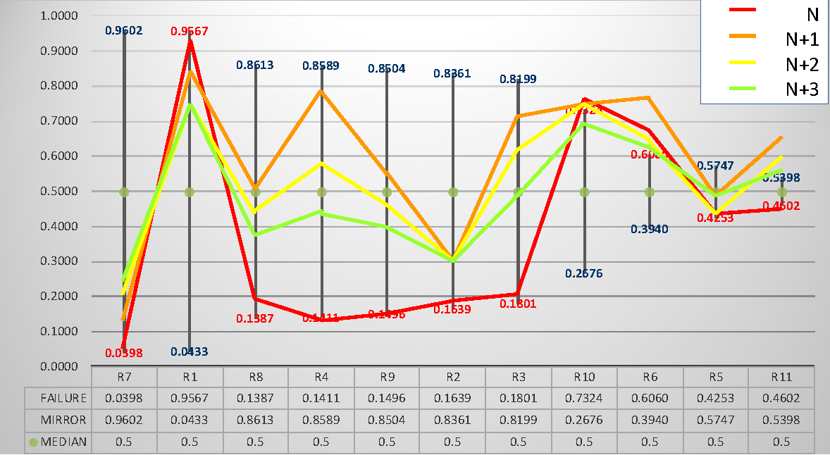
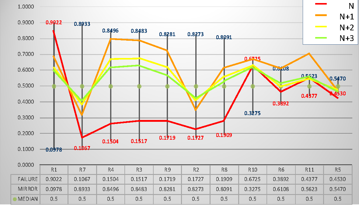
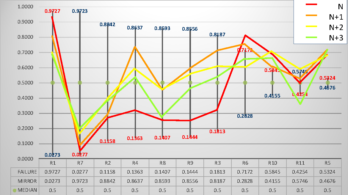
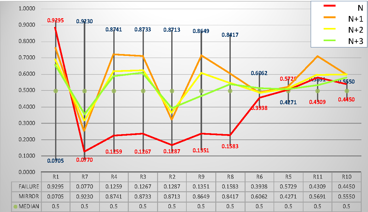
As for the evolution of the business indicators in the postfailure process of reorganization, Figure 1 shows the PDFR frontier of accounting ratios in year N⁷. Note that each vertical line represents the position of a ratio in terms of percentiles, being the red number the percentile in which the median value of the ratio for the group of failed firms is placed. Note also that the ratios are ordered from higher to lower discriminant power as the percentile 0.5 is that of the median value of the ratio for the population under study and the discriminant power is measured by the distance in percentiles between the median of the population (0.5) and the percentile of the median value of the ratio for the group of failed firms (red number). Over this representation of the position of the group of failed firms in respect of the population, called PDFR frontier, we display the position in terms of percentiles of the group of firms under reorganization. The red line characterizes the group of firms with Equity<0 during the year N with three subsequent years of positive equity. We can see that the group of firms under reorganization starts from a situation wherein their ratios are very close to the failure frontier (red numbers). The orange line shows the situation of the group one year later (N+1), the yellow line represents the situation two years later (N+2), and the green line represents the situation three years later (N+3). The results for Finland and Portugal (the countries with the lowest and the highest number of firms in the sample, respectively) have been included in this section, whereas the charts with the results for the other four countries are included in Appendix 5 for brevity.

The first pattern we can see in Figure 1 is that the improvement is the most salient from the red line to the next-year orange line; however, those big changes in the ratios moderate approximately to half during the next two years. However, this is not a general pattern for all the ratios, not even for the most discriminant ones, as one could expect. The two most discriminant ratios (R1, TL/TA and R7, RE/TA) show a small and progressive improvement in all cases, but the improvement is not sufficient to obtain the central value (median) of the population, not even after three years. This result is consistent with the role of debt-to-equity conversion in post-bankruptcy survival identified by Cepec & Grajzl (2020) but also with Ayadi et al. (2020) who find that bankrupt firms maintain high leverage ratios several years after reorganization.

Regarding the second group of ratios, R2 (CA/CL) shows a similar behavior (though improvement is not always progressive), as the evolution during the next three years is far from reaching the central values of the population (except in sector 4 in Germany). The other four ratios in the second group, all of which are representative of profitability and cash flow generation (R3, R4, R8 and R9), have an extraordinary reaction during the first year with better values than the central values of the population (or just close to them in Italy) that is moderated during years two and three and higher (in France, Portugal, and Spain) or even below (in Finland and Germany) the central values of the population.

In every case, the improvement of profitability (R3 and R4) is higher than the improvement of the margin over sales (R9) and especially of the cash flow over total assets (R8). The crucial relevance of return on assets in reorganization processes is consistent with some previous literature (Camacho et al., 2015; Campbell, 1996; Segovia & Camacho, 2012).

The third group of ratios is in general poorly discriminant. As expected, the improvement is not high, and some of them even evolve to a worse situation. For example, in Finland, France, and Germany, R5 and R6 do not show a clear pattern of improvement/worsening, while in Portugal and Spain they improve only slightly.

Changes in asset turnover (R10) are structural. During the reorganization, relevant reductions of assets (Denis & Rodgers, 2007) should affect this feature, but our results only show that relevance for Germany. For sales growth (R11), the first year all sectors and countries (except S1 in France and Germany and sectors three and four in Germany) show an improvement that later moderates during the next two years in the four sectors. The clearer patterns for all ratios in Portugal, Spain, and Italy are due to the large number of firms analyzed to construct the frontier and the high number of firms studied under reorganization.

Figure 1. Evolution of the PDFR Frontier in Finland vs Portugal by Sector for Groups under Reorganization

Panel A. Finland, Sector 1, Manufacturing, Average Group 2010-2013

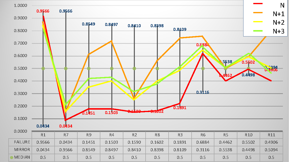
Panel B. Portugal, Sector 1, Manufacturing, Average Group 2010-2013

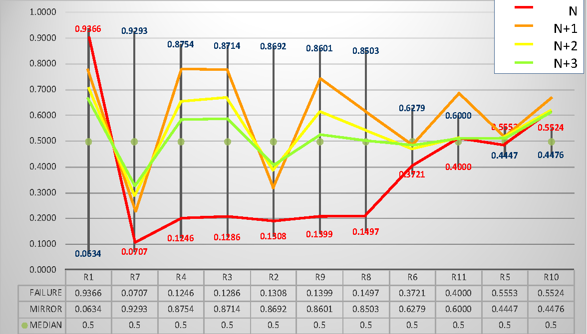
Panel C. Finland, Sector 2, Construction, Average Group 2010-2013

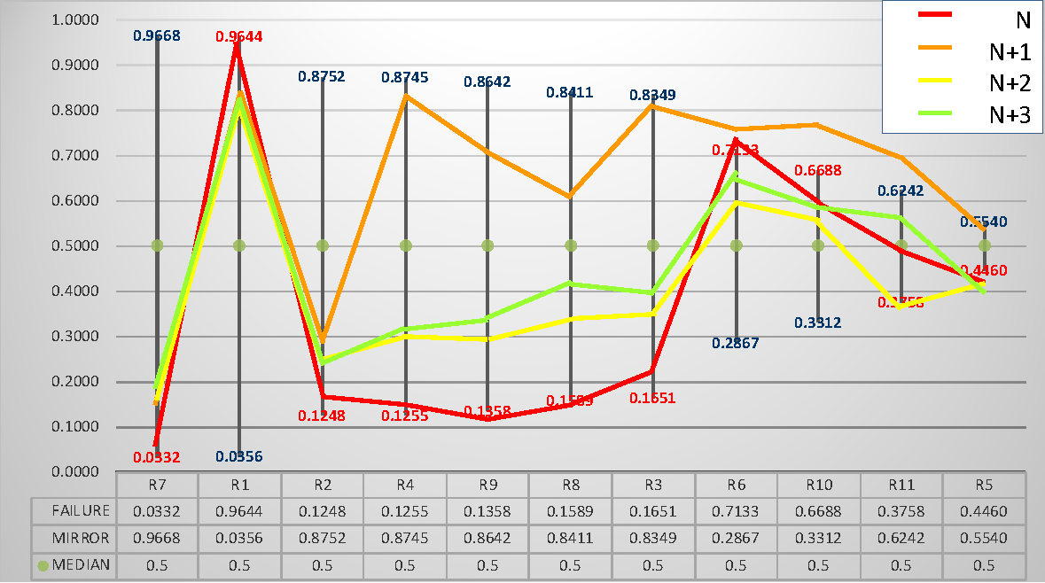
Panel D. Portugal Sector 2, Construction, Average Group 2010-2013

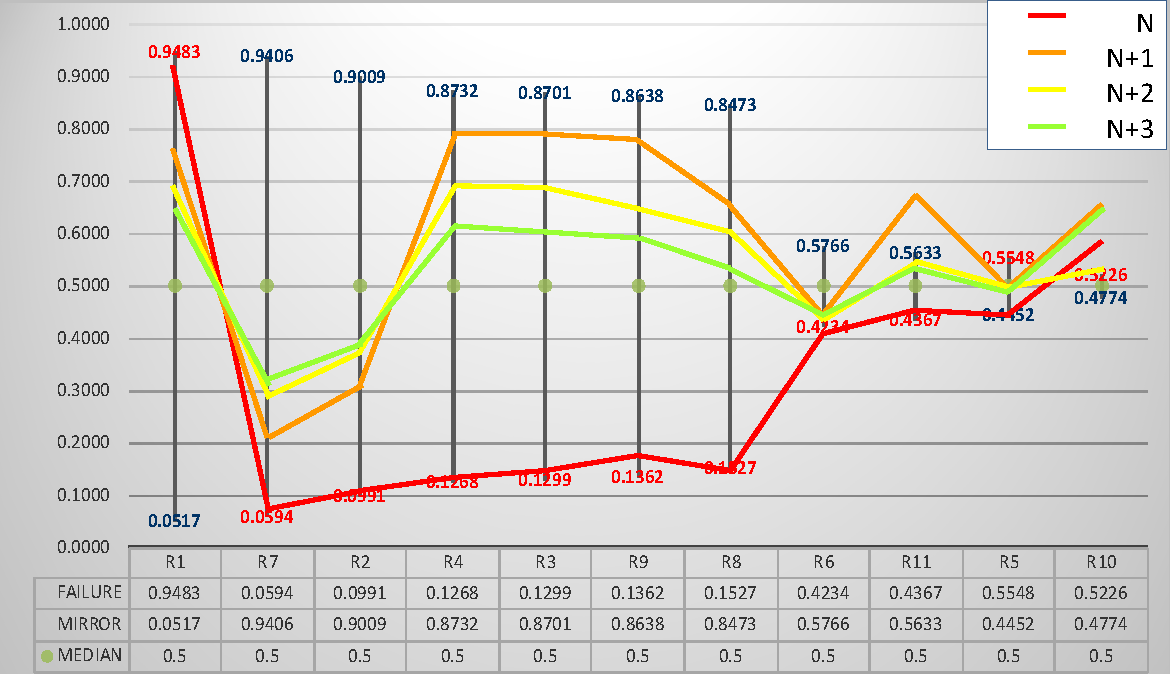
Panel E. Finland, Sector 3, Business Services, Average Group 2010-2013

Panel F. Portugal, Sector 3, Business Services, Average Group 2010-2013

Panel G. Finland, Sector 4, Trade, Average Group 2010-2013

Panel H. Portugal, Sector 4, Trade, Average Group 2010-2013

The application of Boosting to distinguish between the sample of firms under reorganization, and the remainder of failed firms (untabulated) shows the relevance of R1 and R7. Unlike the analysis to differentiate failed and nonfailed firms, all the remaining ratios play a role now in the application of Boosting, and specifically income drivers, such as R3, R4, R8, and R11, become much more discriminant.

4.3. Evolution of failure and postfailure scores

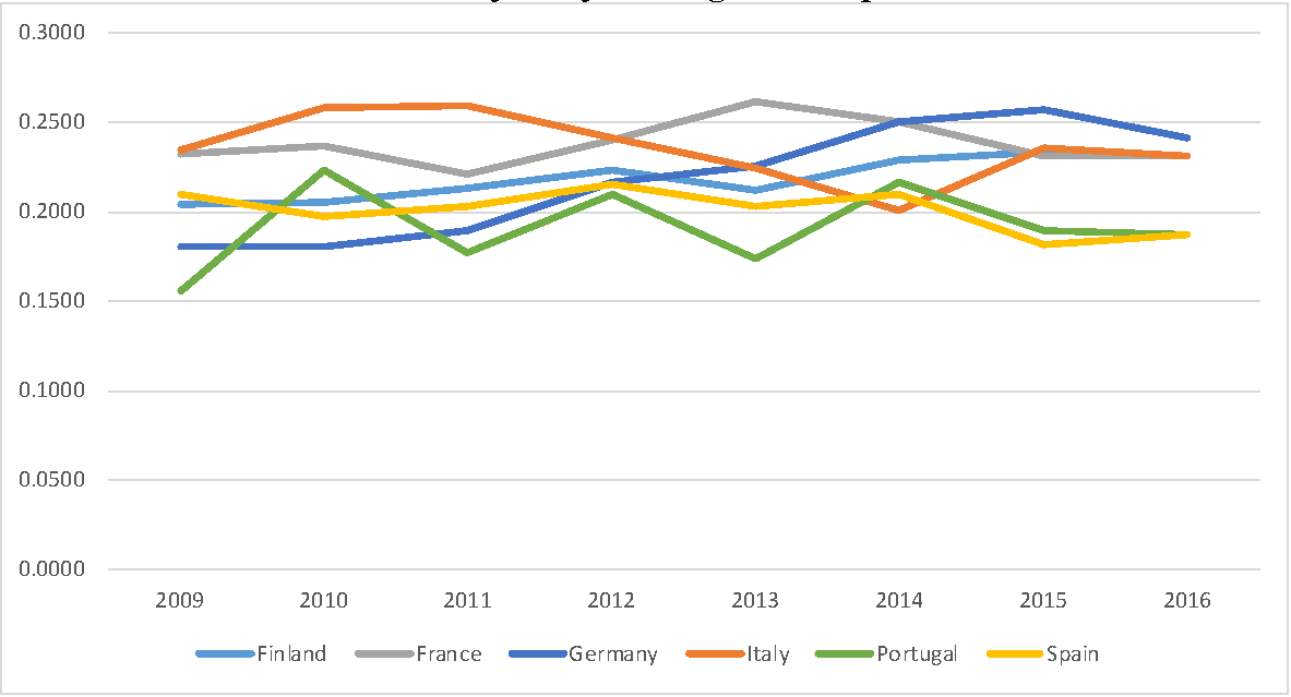
As the PDFR methodology allows us to quantify distances to failure of populations and groups inside those populations, we have computed the scores of the group of failed SMEs with respect to the total population of SMEs by country and year. Figure 2 displays the score \({\overline{S}}^{*}(10,q)\), which is the average score for the most discriminant 10 ratios. We can see that the values range around 0.20-0.25 in most cases during the period analyzed. Gross domestic product was quite stable during the period in the six countries, with a growing trend in Finland and Germany (Appendix 7) that seems to address the evolution of the scores, in a clearer manner in Germany.

Figure 2. PDFR Scores for Failed Firms by Year and Country, Finland, France, Germany, Italy, Portugal, and Spain

Finally, Table 7 shows the average scores obtained by country and sector for the group of firms under reorganization. Blue numbers indicate the score obtained by the total failed firms in that country and sector. The value can be interpreted as the distance to failure of the population as a whole as measured in percentiles. Consider that the median value of the population is 0.5 for each ratio. Given that the PDFR computed is an average for 10 ratios, 0.5 is the benchmark of the population.

The lines with N show the distance to failure of the group of firms under reorganization during the year in which they are failed firms (with equity lower or equal to zero). Using failed firms in 2010, 2011, 2012 and 2013 with three years of positive equity ahead, we computed scores for all of these firms during years N, N+1, N+2, and N+3 followed by average values of the scores. For example, in Finland, we included four groups of firms, namely, the failed group in 2010, the failed group in 2011, the failed group in 2012 and the failed group in 2013, among all firms with positive equities during the next three years.

Table 7. Reorganization. Average PDFR Scores and Distances to Failure by Country and Sector

Sector 1	Finland	France	Germany	Italy	Portugal	Spain
Failed group	0.1880	0.2216	0.1864	0.2755	0.1864	0.2340
N	0.0124	0.0760	-0.0114	-0.0013	0.0629	0.0265
N+1	0.1763	0.2649	0.1533	0.1803	0.2958	0.2604
N+2	0.1021	0.1123	0.1006	0.1778	0.2467	0.2221
N+3	0.1079	0.1650	0.1024	0.1624	0.2267	0.2071
Sector 2	Finland	France	Germany	Italy	Portugal	Spain
Failed group	0.1952	0.2647	0.1942	0.2453	0.1942	0.1868
N	0.0210	0.0770	-0.0025	-0.0026	0.0203	0.0298
N+1	0.2145	0.3180	0.1872	0.1903	0.2557	0.2442
N+2	0.0869	0.1727	0.1449	0.1727	0.2182	0.1981
N+3	0.1090	0.2256	0.1297	0.1752	0.1997	0.1835
Sector 3	Finland	France	Germany	Italy	Portugal	Spain
Failed group	0.2227	0.2200	0.2009	0.2239	0.2009	0.1958
N	0.0077	0.0191	0.0516	0.0070	0.0714	0.0394
N+1	0.1866	0.2166	0.1863	0.1722	0.2631	0.2252
N+2	0.1592	0.1853	0.1364	0.1611	0.2229	0.1890
N+3	0.1372	0.1561	0.1868	0.1605	0.2165	0.1819
Sector 4	Finland	France	Germany	Italy	Portugal	Spain
Failed group	0.2014	0.2430	0.1607	0.2384	0.1607	0.2167
N	0.0483	0.0567	0.0571	0.0001	0.0596	0.0609
N+1	0.1773	0.2315	0.1679	0.1550	0.2397	0.2955
N+2	0.1763	0.1925	0.1367	0.1589	0.2058	0.2388
N+3	0.1137	0.1866	0.1257	0.1606	0.1981	0.2279

Notes: The table displays average scores for the group of failed firms considering 10 ratios in the period 2010-2013. These are the benchmarks by country and sector. The population is made up of 306,447 SMEs. The next four lines show the distances to failure of the groups of firms under reorganization, the year they are failed (N), and the next three years (N+1, N+2, N+3). Definition of the score and the distance computed: $ \overline{S^{*}}(10,q) $ is the average score for failed firms (q) using 10 ratios when the correlation effect is eliminated; and $\overline{D^{*}}(10,a)$ is the average distance to failure for a group a using 10 ratios when the correlation effect is eliminated.

For the four groups, we computed scores for every company that year (N) and the next three years (N+1, N+2, N+3). The benchmark information of the population and the whole group of failed firms is taken in every case in year N (numbers of the total failed group in the population, in blue in Table 7). To synthetize this information, we have integrated the four groups analyzed by country and sector in averages for the period 2010-2013. During the period they are failed (N), the groups of firms under successful reorganization show small differences in respect to the failed firms in every population (by sector and country). A common pattern can be identified along the next three years in all the groups analyzed: the distance to failure remarkably increases during the period N+1 and moderates during the following two periods, which show varied trends across countries and sectors. However, at the end of the third year, no group reaches the central value of the population (0.5) by adding the distance to failure to the score of the failed group. In the best cases, some groups obtain a score close but lower than 0.5 (for example, France in sector 2, starts from a benchmark of 0.2647, and the groups obtain an average distance-to-failure score of 0.2256 for the third year, for a total of 0.4903. This in the only case in which the total score was higher to 0.5 in whatever period: obtaining 0.5827 for N+1). In sum, during these three years, firms under successful reorganization have evolved from a very high failure risk to a moderate failure risk, but no group has evolved to a medium failure risk (vid. Appendix 8) as their distance to failure is not greater than that of the population yet.

In Appendix 7, Panel A, we have included a second version of Table 7. In it only scores have been included. The PDFR scores of the group of failed firms in the population by country and sector (in blue) are followed by the PDFR scores (instead of distances to failure) of the groups under study as failed firms (in year N) and then as successfully reorganized firms along the next three years (N+1, N+2, and N+3). In Panel B of Appendix 7 we include the Z-scores computed for those same groups of firms under reorganization by country and sector. This way, we have compared the evolution of scores applying both methodologies to find out the robustness of our results with the well-known and widely applied Z-scores (Altman, 1977) but also to highlight the additional possibilities of analysis contributed by the PDFR methodology.

The evolution of Z-scores shows a similar pattern across countries and sectors (except the German sector 4), that is, a stronger increase from N to N+1 and moderated increases during the following two periods. Unlike the PDFR scores, there is no decrease of scores from year N+1 to year N+2, and N+3 is the maximum value in every group of firms by country and sector. The reason is the nature of the ratios included and the weighting attributed to them by the Altman's (1977) model⁸. The PDFR model (Figure 1 and Appendix 5) shows that ratios of financial and economic structure evolve in a parsimonious pace whereas ratios related to income, like profitability, profit margin, and cash flow, have a quick reaction the first year that moderates in the next two years in most countries and sectors. However, the Z-score is mainly made up of ratios of structure (3 out of 5), asset turnover shows a very scarce discriminant power, and only a ratio of profitability is affecting the Z-score to show that higher increase from year N to year N+1.

Concerning the scores, we can appreciate that PDFR offers two benchmarks, the median value of the population by country and sector for each ratio, jointly represented in percentiles by 0.5, and the score obtained by the group of all failed firms in the population by country and sector. In the specific period studied we can observe how the groups of firms in the process of reorganization evolve from values close to those of the group of failed firms to the benchmark of the population (0.5) without reaching it. By contrast, the Z-score has a unique benchmark as frontier between failed and healthy firms, common for different countries and sectors. By ignoring the economic and sectoral frameworks in which firms are recovering from failure, we can appreciate tricky scores. For example, German firms in sector 4 would be considered clearly healthy even during the period in which their equity was zero or negative. By contrast, firms belonging to the four sectors in Italy, Portugal, and Spain obtain values of failed firms even after three years with positive equity. The same occurs with Sector 1 in Finland and sector 3 in France. Both methods computing scores demonstrate ability to register the firms' improvement, but PDFR identifies the contribution by each ratio to that recovery measured in statistical percentiles.

5. Conclusions

This paper analyzes the behavior of several financial indicators (traditionally found as discriminant to identify failed firms) during successful reorganization to check if the basic forces behind failure and reorganization are relatively stable across time, countries, and sectors. Using PDFR the influence of uncontrollable environmental conditions is neutralized by eliminating the year, country, and sector biases by comparing with benchmarks to focus mainly on firm's performance differences.

In this way, we measure how far the group of firms under reorganization are from the benchmarks by year, country, and sector, and their evolution during the subsequent process of recovery, for the population of SMEs in Finland, France, Germany, Italy, Portugal, and Spain during the period 2009 to 2016 and considering the sectors of manufacturing, construction, business services and trade. Our results show that once the biases due to the macroeconomic and the sectoral frameworks have been neutralized the financial indicators behind the difference between failed and nonfailed firms can be classified into three groups according to their discriminant power. The first group of financial structure variables that includes two ratios is the most discriminant for all countries and sectors analyzed. A second group of variables mainly related to return on assets, margin, cash flow, and working capital is powerfully discriminant, although the order of the variables changes from country to country and from sector to sector. The third group consists of the four variables with lower discriminant power across countries and sectors. The order of the three groups is consistent across years, countries, and sectors. Furthermore, in contrast to our expectations, we find more homogeneous results across sectors inside every country than across countries inside every sector. This result seems to contradict the generally accepted industry effect. However, remarkable differences in the stage of the economic cycle and the financial setting by country, derived from the deep financial crises included in the period under study, have originated differences in the stages of the industry cycles across countries, in line with the reasoning provided by Chang & Dasgupta (2002), Goddard et al. (2009), and Rajan & Zingales (1998).

Second, the features that the firms under reorganization improve first are not the most discriminant ones. In fact, indebtedness and retained earnings to total assets show a slow and progressive pattern of improvement in all countries and sectors. Current assets to current liabilities also show a slow pattern of improvement that is not always progressive. Profitability measures are the factors that quickly and strongly improve during the first year in all countries and sectors, but the improvement moderates considerably during years two and three. The same pattern, albeit not as strong, is found for margin, cash flow to assets and sales growth. The latter exhibits a more moderate effects as it belongs to the third group of variables (less discriminant). Finally, current assets to total assets, assets turnover and financial expenses to total liabilities do not show clear patterns or slight improvements in all sectors. Our results indicate a clear first reaction of income measures that is stronger during the first period, and then moderates during periods two and three, and a progressive but slow change in structure or economic-financial position.

Regarding the scores, we have found that along the period studied, the average scores computed with 10 ratios by country converge around 0.20-0.25. Using PDFR, we have quantified in statistical percentiles (which is a homogeneous, comparable, and understandable measure) how far the group of failed firms is located from the median values of the population based on country and sector, and then we computed how the selected groups under reorganization increase (or reduce) their distances to failure year after year. Unlike the well-known Z-score, for which only one benchmark is used to distinguish failed from healthy firms for whatever country, sector, and period, PDFR scores are evaluated against two benchmarks: the score of the failed firms, and the score of the population, both ones computed by country, sector, and period. In the current study, the results show that both methods capture the firms' improvement but only PDFR neutralizes the bias produced by the macroeconomic and sectoral frameworks.

A relevant result is that after three years of positive equity, no group has obtained the central values of the population as a global result, even if our analysis of the variables evolution shows that those central values are by far obtained for income variables already during the first year. The recovery of the economic-financial position of the firm seems to take a period longer than three years after a period of failure. This finding is consistent with the learning process after failure and the derived modification of the firm's norms, strategies and objectives (Mayr et al., 2017) with new methods of managing cash, investment, stakeholder relationships, and growth as well as new understandings of the marketplace and competition (Ucbasaran et al., 2013).

Our results are of interest for analysts, researchers and academics concerned with the effect of macroeconomic and sectoral environments on the SMEs' financial performance; but especially these findings on the behavior of SMEs under reorganization are of interest for investors, creditors, regulators, and public administration, as stakeholders concerned with the capacity of close-to-failure SMEs to recover.

Some limitations of the study must be recognized. First, the access to SMEs' data is restricted to the information available in the database used and some bias could derive from the criteria of inclusion applied in every country. Second, the selection of an accounting definition for the categorization of failed firms is affected by the endogeneity problem present in the relationship between many accounting variables, as explained in section 3.1. Third, this study is performed for the period subsequent to a serious financial crisis (started in 2007-2008) suffered in all the countries included in the analysis and the recovery of those countries have followed not homogeneous patterns as our results clearly show. This specific macroeconomic framework could be addressing the results concerning the country-wide effects. Possible extensions of this study can cope with these limitations by using alternative data sources, other definitions of failure/reorganization, different periods, and other countries or geographical regions. In addition, the PDFR methodology can be used for the search of patterns in financial indicators in all other areas of firms' financial performance.

 

---

Appendixes

 

Appendix 1. Variables

Name	Definition
R1=TL/TA	Total Liabilities to Total Assets (long-term solvency risk, book leverage ratio)
R2=CA/CL	Current Assets to Current Liabilities
R3=EBIT/TA	Earnings Before Interests and Taxes to Total Assets
R4=NI/TA	Net Income to Total Assets (profitability, return on assets)
R5=CA/TA	Current Assets to Total Assets
R6=FE/TL	Financial Expenses to Total Liabilities
R7=RE/TA	Retained Earnings (non distributed benefits) to Total Assets
R8=CF/TL	CashFlow (net income plus amortization and depreciation) to Total Liabilities
R9=NI/Sales	Net Income to Sales
R10=Sales/TA	Sales to Total Assets
R11=growSL	Sales growth, Sales of year (t) minus Sales of year (t-1) divided by Sales of year (t-1)

Appendix 2. Mean and Median Analyses and Tests of Differences, Rest of Countries

Panel A. Finland
Variables	N (NF)	mean (NF)	p50 (NF)	N (F)	mean (F)	p50 (F)	test mean	test median
R1_TL_TA	26550	0.5331	0.5471	2189	1.9673	1.2260	0.0000	0.0000
R2_CA_CL	32264	4.3709	1.8114	2269	1.0970	0.7684	0.0000	0.0000
R3_EBIT_TA	32421	0.1069	0.0917	2284	-0.0892	-0.0122	0.0000	0.0000
R4_NI_TA	32421	0.0760	0.0686	2284	-0.1518	-0.0488	0.0000	0.0000
R5_CA_TA	32422	0.6302	0.6715	2282	0.5846	0.6058	0.0000	0.0000
R6_FE_TL	25138	0.0338	0.0180	2141	0.0318	0.0265	0.4892	0.0000
R7_RE_TA	32423	0.4582	0.4625	2284	-1.2499	-0.3249	0.0000	0.0000
R8_NI_Am_TL	25026	0.5095	0.2430	1983	0.0066	0.0232	0.0000	0.0000
R9_NI_Sales	32086	0.1994	0.0386	2256	-0.1701	-0.0238	0.0001	0.0000
R10_Sales_TA	32148	2.1151	1.7450	2265	3.3663	2.4464	0.0000	0.0000
R11_growSL	27923	0.2382	0.0244	1963	0.1525	-0.0179	0.1694	0.0000
Panel B. France
Variables	N (NF)	mean (NF)	p50 (NF)	N (F)	mean (F)	p50 (F)	test mean	test median
R1_TL_TA	39918	0.5508	0.5533	1130	1.4669	1.2187	0.0000	0.0000
R2_CA_CL	39902	-10.2690	1.5908	1129	0.6935	0.6361	0.9135	0.0000
R3_EBIT_TA	38910	0.0676	0.0556	1113	-0.0951	-0.0236	0.0000	0.0000
R4_NI_TA	38909	0.0542	0.0458	1113	-0.1033	-0.0266	0.0000	0.0000
R5_CA_TA	39918	0.7580	0.8285	1130	0.6796	0.7585	0.0000	0.0000
R6_FE_TL	38902	0.0163	0.0079	1113	0.0159	0.0093	0.7521	0.0026
R7_RE_TA	39918	0.3623	0.3570	1130	-0.6130	-0.3342	0.0000	0.0000
R8_NI_Am_TL	38438	0.2112	0.1513	1078	-0.0299	0.0095	0.0000	0.0000
R9_NI_Sales	38891	-0.0122	0.0257	1107	-0.2211	-0.0111	0.1388	0.0000
R10_Sales_TA	38904	1.9935	1.8020	1112	2.9406	2.5250	0.0000	0.0000
R11_growSL	33903	0.0611	0.0153	947	0.0375	-0.0203	0.3933	0.0000
Panel C. Germany
Variables	N (NF)	mean (NF)	p50 (NF)	N (F)	mean (F)	p50 (F)	test mean	test median
R1_TL_TA	50564	0.6224	0.6574	3844	1.9268	1.2311	0.0000	0.0000
R2_CA_CL	42132	586.9420	1.9359	2798	45.8461	0.9071	0.2134	0.0000
R3_EBIT_TA	35049	0.0975	0.0790	953	0.0129	0.0364	0.0000	0.0000
R4_NI_TA	35544	0.0614	0.0477	983	-0.1049	0.0020	0.0000	0.0000
R5_CA_TA	50564	0.7192	0.7694	3844	0.7032	0.7830	0.0003	0.1064
R6_FE_TL	35190	0.0277	0.0226	989	0.0369	0.0327	0.0000	0.0000
R7_RE_TA	50015	0.2778	0.2341	3829	-1.3577	-0.3707	0.0000	0.0000
R8_NI_Am_TL	34651	0.2398	0.1529	932	0.0115	0.0376	0.0000	0.0000
R9_NI_Sales	11244	-0.2593	0.0190	514	-0.2268	0.0033	0.8792	0.0000
R10_Sales_TA	15845	3.7017	2.1471	1293	3.6231	2.6552	0.8862	0.0000
R11_growSL	11694	0.0734	0.0194	849	0.6487	0.0000	0.3001	0.0000
Panel D. Italy
Variables	N (NF)	mean (NF)	p50 (NF)	N (F)	mean (F)	p50 (F)	test mean	test median
R1_TL_TA	552693	0.7010	0.7544	15515	1.3266	1.0836	0.0000	0.0000
R2_CA_CL	552462	11.0023	1.3715	15504	3.8450	0.8898	0.1320	0.0000
R3_EBIT_TA	552693	0.0530	0.0400	15515	-0.1184	-0.0440	0.0000	0.0000
R4_NI_TA	552654	0.0210	0.0097	15513	-0.1631	-0.0731	0.0000	0.0000
R5_CA_TA	552693	0.7209	0.7979	15515	0.7052	0.7933	0.0000	0.0000
R6_FE_TL	552683	0.0193	0.0133	15515	0.0227	0.0181	0.0000	0.0000
R7_RE_TA	552693	0.2415	0.1844	15515	-0.4152	-0.1483	0.0000	0.0000
R8_NI_Am_TL	545675	0.1474	0.0590	14722	-0.0641	-0.0312	0.0000	0.0000
R9_NI_Sales	551206	0.8839	0.0094	15427	-2.7522	-0.0688	0.2649	0.0000
R10_Sales_TA	552662	1.2551	1.0850	15514	1.5334	1.1558	0.0000	0.0000
R11_growSL	482463	-5.8751	0.0101	13402	0.3142	-0.0359	0.1121	0.0000
Panel E. Portugal
Variables	N (NF)	mean (NF)	p50 (NF)	N (F)	mean (F)	p50 (F)	test mean	test median
R1_TL_TA	733375	0.5384	0.5715	146191	3.3923	1.4785	0.0000	0.0000
R2_CA_CL	729334	342.6442	2.1560	145608	96.1111	0.7024	0.2442	0.0000
R3_EBIT_TA	732805	0.0427	0.0361	145933	-0.3447	-0.1111	0.0000	0.0000
R4_NI_TA	732731	0.0215	0.0189	145927	-0.3883	-0.1259	0.0000	0.0000
R5_CA_TA	733377	0.7324	0.8183	146191	0.7053	0.8168	0.0000	0.0007
R6_FE_TL	502331	0.1408	0.0137	83733	0.0143	0.0074	0.2704	0.0000
R7_RE_TA	733377	0.3036	0.2800	146179	-3.1167	-0.7092	0.0000	0.0000
R8_NI_Am_TL	664466	7.3401	0.1162	118900	-0.0765	-0.0442	0.2201	0.0000
R9_NI_Sales	721623	-0.0420	0.0183	141608	-73.7130	-0.1230	0.3132	0.0000
R10_Sales_TA	721689	1.3877	1.0403	141601	3.4258	1.3039	0.0516	0.0000
R11_growSL	625403	230.7425	0.0009	126367	0.3153	-0.0233	0.3167	0.0000
Panel F. Spain
Variables	N (NF)	mean (NF)	p50 (NF)	N (F)	mean (F)	p50 (F)	test mean	test median
R1_TL_TA	802070	0.5355	0.5548	71641	2.1445	1.2688	0.0000	0.0000
R2_CA_CL	801412	70.8173	1.6661	71612	1.5271	0.5705	0.1164	0.0000
R3_EBIT_TA	802062	0.0307	0.0276	71643	-0.2370	-0.0524	0.0000	0.0000
R4_NI_TA	801874	0.0155	0.0121	71630	-0.2766	-0.0595	0.0000	0.0000
R5_CA_TA	802114	0.6390	0.6907	71645	0.5819	0.6176	0.0000	0.0000
R6_FE_TL	720380	0.3086	0.0179	60459	0.0171	0.0098	0.2389	0.0000
R7_RE_TA	802115	0.3514	0.3272	71645	-1.4687	-0.3788	0.0000	0.0000
R8_NI_Am_TL	739916	-2.5546	0.0821	56433	-0.0379	-0.0158	0.1529	0.0000
R9_NI_Sales	790011	-2.9696	0.0102	70955	-3.7338	-0.0533	0.8550	0.0000
R10_Sales_TA	790228	1.4688	1.1565	70965	2.2695	1.2639	0.0000	0.0000
R11_growSL	688321	0.7427	0.0024	62658	2.7009	-0.0309	0.4401	0.0000

 

Appendix 3. Correlation Matrices by Country

Panel A. Finland
	Failure	R1	R2	R3	R4	R5	R6	R7	R8	R9	R10	R11
Failure	1
R1	0.2345*	1
R2	-0.0328*	-0.0416*	1
R3	-0.1099*	-0.1617*	0.0051	1
R4	-0.1301*	-0.3351*	0.0119	0.9465*	1
R5	-0.0409*	-0.0186*	0.0746*	0.0632*	0.0557*	1
R6	-0.0013	-0.006	0.3630*	0.0039	-0.0083	-0.0026	1
R7	-0.2535*	-0.9772*	0.0369*	0.2179*	0.3687*	0.0169*	0.0054	1
R8	-0.0742*	-0.1778*	0.3650*	0.2343*	0.2463*	0.0211*	-0.0125	0.1737*	1
R9	-0.0059	-0.0181*	0.0139	0.0125	0.0161*	0.002	-0.0026	0.0096	0.0448*	1
R10	0.0773*	0.0381*	-0.0673*	-0.5701*	-0.5453*	0.1171*	0.0199*	-0.0723*	-0.0742*	-0.0052	1
R11	-0.0031	-0.0041	0.0149	0.0086	0.0076	0.0064	-0.0026	0.0027	0.0101	-0.0009	0.0046	1
Panel B. France
	Failure	R1	R2	R3	R4	R5	R6	R7	R8	R9	R10	R11
Failure	1
R1	0.5379*	1
R2	0.0001	-0.0032	1
R3	-0.1881*	-0.2097*	0.0016	1
R4	-0.2098*	-0.2209*	0.0011	0.8637*	1
R5	-0.0585*	-0.0686*	-0.0033	0.0712*	0.0690*	1
R6	-0.0008	-0.0349*	0.0002	-0.0160*	-0.0779*	-0.0795*	1
R7	-0.5337*	-0.9192*	0.0023	0.2520*	0.2615*	0.1074*	0.0133*	1
R8	-0.0925*	-0.2734*	0.0019	0.4951*	0.5620*	-0.0035	-0.0123	0.2668*	1
R9	-0.004	-0.0087	0	0.0654*	0.0709*	0.0119	0.0094	0.0093	0.0572*	1
R10	0.1265*	0.2813*	0.0014	0.0542*	0.0222*	0.1938*	-0.0454*	-0.2479*	-0.0502*	0.0082	1
R11	-0.0039	0.0111	0.0004	0.0445*	0.0355*	-0.0013	0.0054	-0.0091	0.0153*	0.0062	0.0068	1
Panel C. Germany
	Failure	R1	R2	R3	R4	R5	R6	R7	R8	R9	R10	R11
Failure	1
R1	0.1719*	1
R2	-0.0015	-0.0017	1
R3	-0.1090*	-0.1575*	-0.0044	1
R4	-0.1119*	-0.1755*	-0.0017	0.4356*	1
R5	-0.0183*	0.002	-0.0019	0.1002*	0.0457*	1
R6	0.0118	0.002	-0.0006	-0.0033	-0.3962*	-0.0277*	1
R7	-0.0936*	-0.9633*	0.0008	0.1686*	0.3453*	-0.0022	-0.0446*	1
R8	-0.0802*	-0.3797*	-0.0049	0.4877*	0.4112*	-0.0282*	-0.2158*	0.3928*	1
R9	0.0004	0.0256*	0.0005	0.1519*	0.0628*	-0.0171	0.0014	0.0298*	0.2341*	1
R10	-0.0003	0.0043	-0.0007	0.0527*	0.0084	0.0087	0.0271*	-0.0012	0.0035	0.0087	1
R11	0.0337*	0.0079	0.0005	0.0086	0.0039	0.0055	-0.0002	-0.0118	-0.0034	0.0004	0.0001	1
Panel D. Italy
	Failure	R1	R2	R3	R4	R5	R6	R7	R8	R9	R10	R11
Failure	1
R1	0.1238*	1
R2	-0.0004	-0.0005	1
R3	-0.1730*	-0.4825*	0.0007	1
R4	-0.1735*	-0.4960*	0.0004	0.8530*	1
R5	-0.0102*	0.0430*	-0.0003	0.0807*	0.0502*	1
R6	0.0018	-0.0024	0.0034*	-0.0145*	-0.0230*	-0.0104*	1
R7	-0.1214*	-0.9941*	0.0004	0.5008*	0.5143*	-0.0366*	-0.0004	1
R8	-0.0028	-0.0146*	0.0067*	0.0199*	0.1308*	-0.0002	0.3391*	0.0089*	1
R9	-0.0013	-0.0005	0	0.0031	0.0029	-0.0008	-0.0002	0.0009	0.0001	1
R10	0.0420*	0.0995*	0.0004	0.0695*	0.0106*	0.2616*	-0.002	-0.1034*	0.0103*	-0.002	1
R11	0.0004	-0.0006	0	0.0007	0.0001	-0.0017	0	0.0004	0	0	0.0017	1
Panel E. Portugal
	Failure	R1	R2	R3	R4	R5	R6	R7	R8	R9	R10	R11
Failure	1
R1	0.0437*	1
R2	-0.0006	0	1
R3	-0.0097*	0.0283*	0	1
R4	-0.0124*	0.0194*	0	0.9988*	1
R5	-0.0241*	-0.0183*	0.001	0.0445*	0.0558*	1
R6	-0.0006	-0.0003	0.0087*	0.0001	0	-0.0009	1
R7	-0.0293*	-0.6376*	0	-0.7622*	-0.7475*	0.0127*	0.0001	1
R8	-0.0006	-0.0001	0.9859*	0.0002	0.0002	0.0006	0.9839*	0.0002	1
R9	-0.0025	-0.0005	0	0.0003	0.0004	-0.0007	0	0.0001	0.0001	1
R10	0.0047*	0.1901*	0	0.9712*	0.9608*	-0.0045*	-0.0003	-0.9606*	-0.0005	0	1
R11	-0.0005	-0.0001	0	0	0	-0.0013	0	0	0	0	0	1
Panel F. Spain
	Failure	R1	R2	R3	R4	R5	R6	R7	R8	R9	R10	R11
Failure	1
R1	0.0303*	1
R2	-0.0005	-0.0001	1
R3	-0.0244*	-0.8593*	0	1
R4	-0.0172*	-0.6073*	0	0.9160*	1
R5	-0.0575*	0.0014	0.0014	0.001	-0.0005	1
R6	-0.0004	-0.0004	0.0053*	-0.0001	-0.0002	-0.0021	1
R7	-0.0262*	-0.8605*	0.0001	0.9780*	0.9211*	-0.0003	0.0001	1
R8	0.0004	0.0005	-0.8486*	0.0002	0.0001	-0.0013	-0.2020*	-0.0001	1
R9	-0.0001	0	0	0.0001	0.0001	0.0014	-0.0004	0	0.0003	1
R10	0.0376*	0.5573*	-0.0003	-0.7861*	-0.8507*	0.0630*	-0.0004	-0.8184*	0.0004	0.0004	1
R11	0.0024	0	0	0.0001	0	0.0004	0	0	0	0	-0.0006	1

Appendix 4. Variable Order with Boosting by Country and Sector to Explain Failure

Panel A. Finland
Variables	Total	Total	S1	S1	S2	S2	S3	S3	S4	S4
R1	1	-	1	-	1	-	1	-	1	-
R7	5	2		2	5	2	4	2	2	2
R2	3	3		3	4	4	5	3		3
R3	4	8		7	3	8	3	9		10
R4	10	10		11	8	10	11	11		11
R8	6	9		9	8	11	10	5	2	9
R9	11	11		10		9	9	8		8
R5	7	6		8	7	7	7	4		5
R6	8	4		4	2	5	7	6		6
R10	2	7		6	6	3	2	7		4
R11	8	5		5	10	6	6	10		7
Panel B. France
Variables	Total	Total	S1	S1	S2	S2	S3	S3	S4	S4
R1	1	-	1	-	1	-	1	-	1	-
R7	2	2		2		2	3	2	2	2
R2	4	3		3		4	2	3		3
R3	6	11		6		10	5	11		9
R4	5	5		8		11	7	5		6
R8		9		7		9	9	4		11
R9	3	8		10		7	6	6		10
R5		4		5		3		7		4
R6		6		4		5	8	8		7
R10		7		11		8		9		5
R11		10		9		6	4	10		8
Panel C. Germany
Variables	Total	Total	S1	S1	S2	S2	S3	S3	S4	S4
R1	1	-	1	-	1	-	1	-	1	-
R7		2		2	2	2		2		2
R2		3		3		6		3		6
R3		9		7		8		7		9
R4		11		10	4	11		11		11
R8		4		5		3		5		8
R9		7		8	4	10		10		10
R5		5		9	3	4	2	4		4
R6		8		6		9		6		3
R10		6		4		7		9		5
R11		10		11		5		8	2	7
Panel D. Italy
Variables	Total	Total	S1	S1	S2	S2	S3	S3	S4	S4
R1	1	-	1	-	1	-	1	-	1	-
R7	2	2	2	2	2	2	2	2		2
R2	4	3	4	3	3	4	5	3		3
R3	3		3			8	7			8
R4		5	4	4		7		5		4
R8	7	6	4	5		5	3	6		6
R9		4	4	6		3		4		7
R5	5	7	4	7		9	5	7		5
R6	6		4			10	3			9
R10	7					6	9
R11	7					11	7
Panel E. Portugal
Variables	Total	Total	S1	S1	S2	S2	S3	S3	S4	S4
R1	1	-	1	-	1	-	1	-	1	-
R7	2	2	2	3		2		2	2	2
R2	3	4	3	2		3		3		3
R3				7		9				6
R4		5		5		7		5		5
R8		3		4		5		4		4
R9				9		4
R5				8		6				6
R6				6		8				6
R10
R11			3
Panel F. Spain
Variables	Total	Total	S1	S1	S2	S2	S3	S3	S4	S4
R1	1	-	1	-	1	-	1	-	1	-
R7	2	2		2	2	2	3	2		2
R2		3		3		3		3		3
R3
R4				7
R8	4	5		5		5		5	2
R9
R5	3	4		4		4	2	4		4
R6				6		6		6
R10						7
R11

Appendix 5. Evolution of the PDFR frontier in France, Germany, Italy, and Spain by sector for groups under reorganization

Panel A.1. France, Sector 1, Manufacturing, Average Group 2010-13

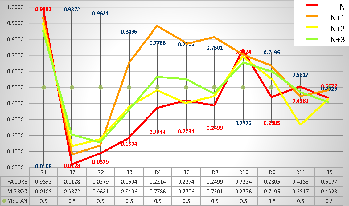
Panel A.2. France, Sector 2, Construction, Average Group 2010-13

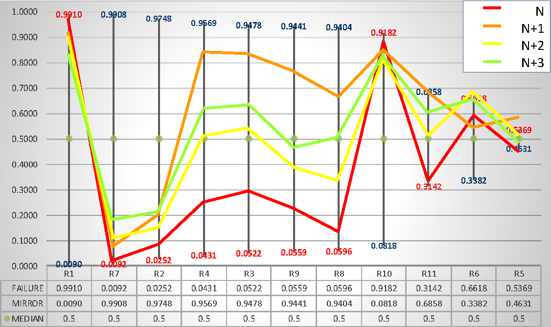
Panel A.3. France, Sector 3, Business Services, Average Group 2010-13

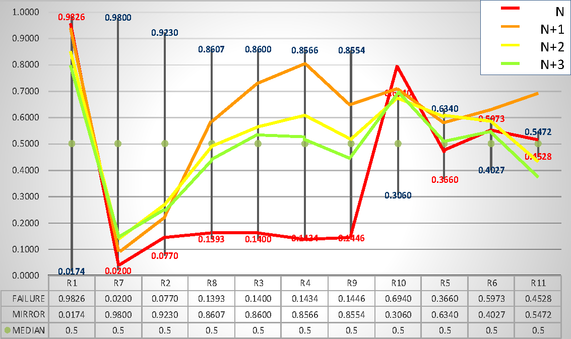
Panel A.4. France, Sector 4, Trade, Average Group 2010-13

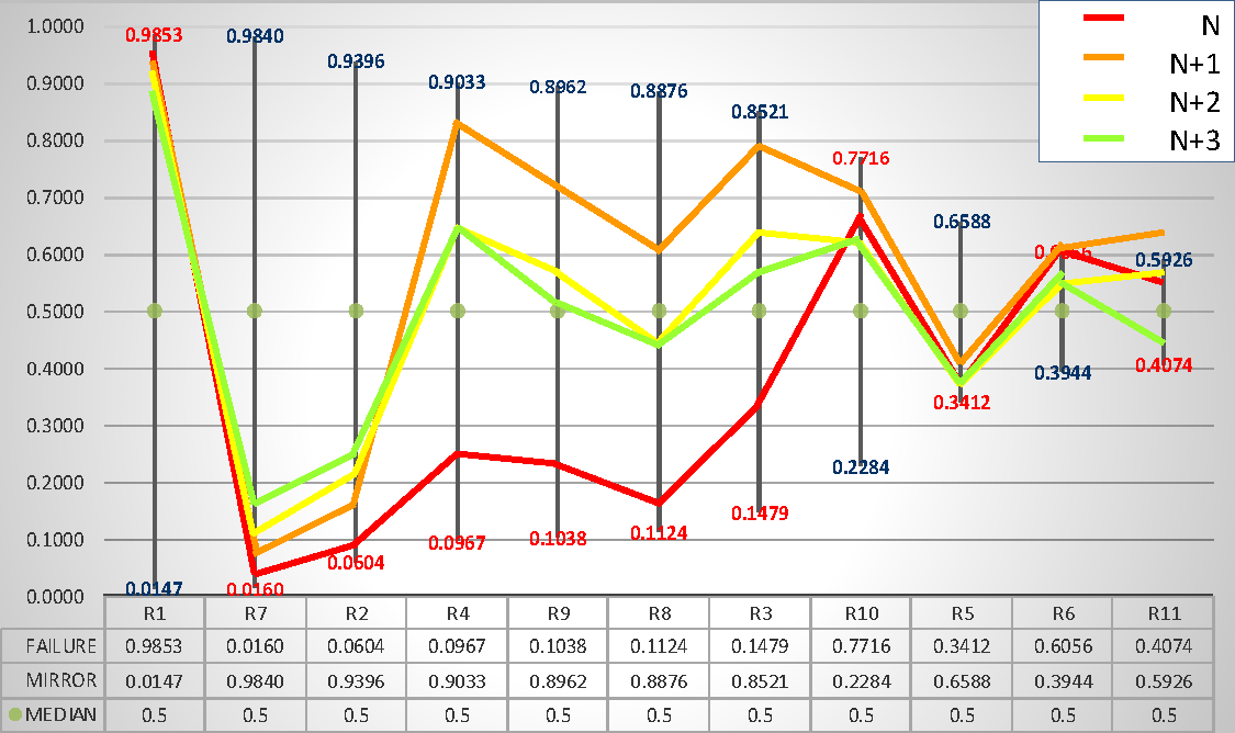
Panel B.1. Germany, Sector 1, Manufacturing, Average Group 2010-13

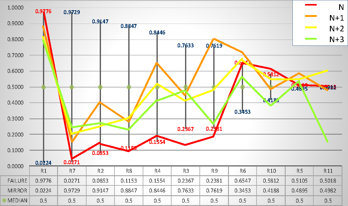
Panel B.2. Germany, Sector 2, Construction, Average Group 2010-13

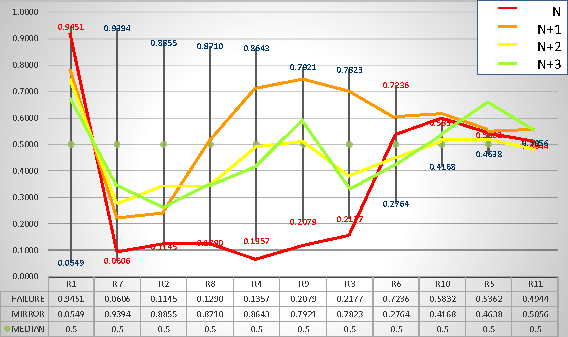
Panel B.3. Germany, Sector 3, Business Services, Average Group 2010-13

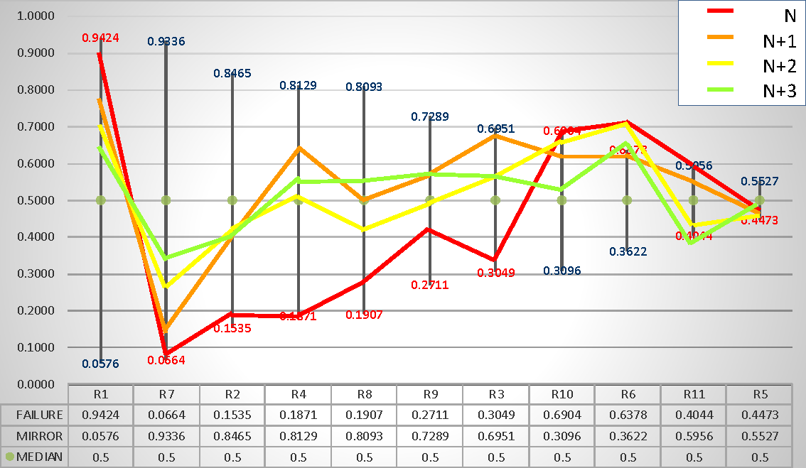
Panel B.4. Germany, Sector 4, Trade, Average Group 2010-13

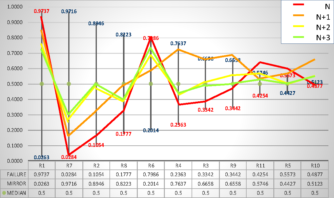
Panel C.1. Italy, Sector 1, Manufacturing, Average Group 2010-13

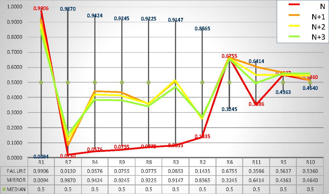
Panel C.2. Italy, Sector 2, Construction, Average Group 2010-13

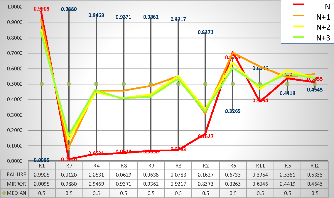
Panel C.3. Italy, Sector 3, Business Services, Average Group 2010-13

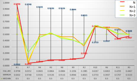
Panel C.4. Italy, Sector 4, Trade, Average Group 2010-13

Panel D.1. Spain, Sector 1, Manufacturing, Average Group 2010-2013

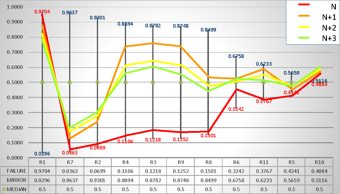
Panel D.2. Spain, Sector 2, Construction, Average Group 2010-2013

>

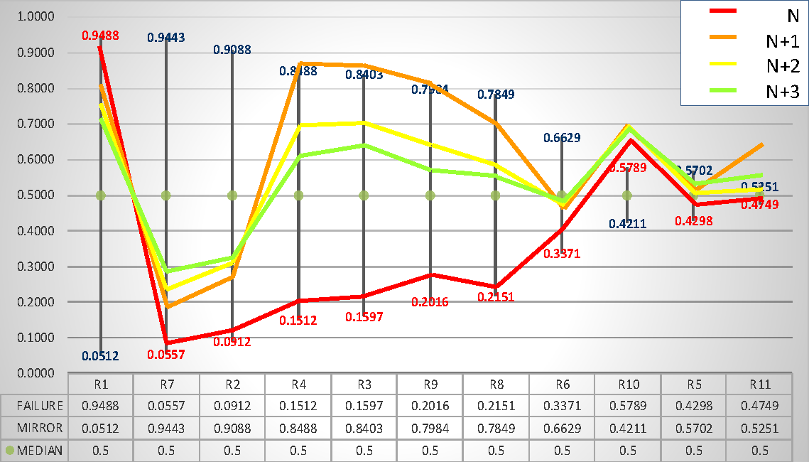
Panel D.3. Spain, Sector 3, Business Services, Average Group 2010-2013

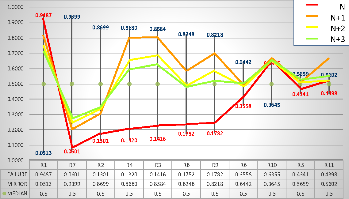
Panel D.4. Spain, Sector 4, Trade, Average Group 2010-2013

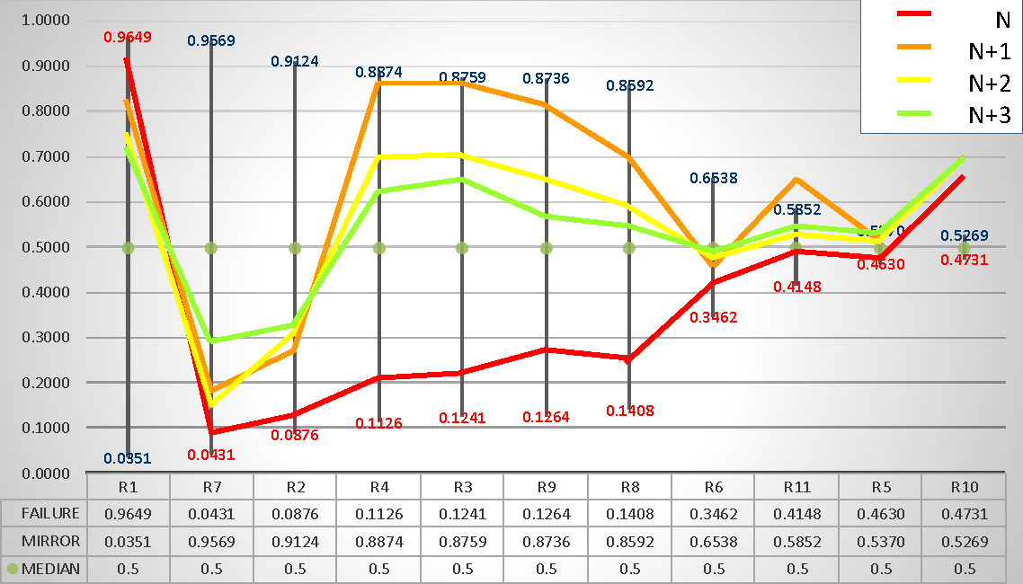
Appendix 6. Evolution of GDP in the Six Countries for the Period 2006-2016

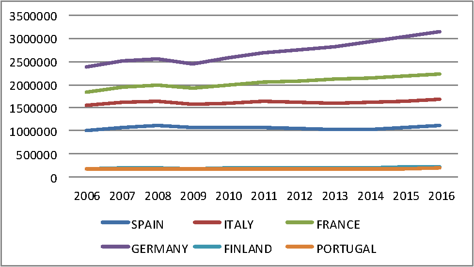
Appendix 7.

Panel A. Reorganization. Average PDFR Scores by Country and Sector
Sector 1	Finland	France	Germany	Italy	Portugal	Spain
Failed group	0.1880	0.2216	0.1864	0.2755	0.1864	0.2340
N	0.2003	0.2977	0.1749	0.2743	0.2493	0.2606
N+1	0.3643	0.4866	0.3397	0.4558	0.4821	0.4944
N+2	0.2901	0.3340	0.2869	0.4533	0.4330	0.4561
N+3	0.2959	0.3867	0.2888	0.4379	0.4130	0.4411
Benchmark	0.5000	0.5000	0.5000	0.5000	0.5000	0.5000
Sector 2	Finland	France	Germany	Italy	Portugal	Spain
Failed group	0.1952	0.2647	0.1942	0.2453	0.1942	0.1868
N	0.2162	0.3417	0.1917	0.2428	0.2145	0.2166
N+1	0.4097	0.5827	0.3814	0.4357	0.4499	0.4309
N+2	0.2821	0.4374	0.3391	0.4180	0.4124	0.3849
N+3	0.3042	0.4903	0.3239	0.4205	0.3939	0.3703
Benchmark	0.5000	0.5000	0.5000	0.5000	0.5000	0.5000
Sector 3	Finland	France	Germany	Italy	Portugal	Spain
Failed group	0.2227	0.2200	0.2009	0.2239	0.2009	0.1958
N	0.2304	0.2391	0.2525	0.2309	0.2723	0.2352
N+1	0.4093	0.4366	0.3872	0.3960	0.4640	0.4210
N+2	0.3819	0.4053	0.3373	0.3850	0.4237	0.3847
N+3	0.3599	0.3761	0.3877	0.3843	0.4174	0.3777
Benchmark	0.5000	0.5000	0.5000	0.5000	0.5000	0.5000
Sector 4	Finland	France	Germany	Italy	Portugal	Spain
Failed group	0.2014	0.2430	0.1607	0.2384	0.1607	0.2167
N	0.2497	0.2997	0.2178	0.2385	0.2203	0.2776
N+1	0.3787	0.4745	0.3287	0.3934	0.4005	0.5122
N+2	0.3777	0.4356	0.2974	0.3973	0.3665	0.4555
N+3	0.3150	0.4297	0.2864	0.3990	0.3588	0.4446
Benchmark	0.5000	0.5000	0.5000	0.5000	0.5000	0.5000
Panel B. Reorganization. Average Z-scores by Country and Sector
Sector 1	Finland	France	Germany	Italy	Portugal	Spain
Failure benchmark	1.8100	1.8100	1.8100	1.8100	1.8100	1.8100
N	0.9768	0.6860	1.3138	0.5271	-0.4368	-0.3602
N+1	1.2969	1.5332	1.8124	0.9960	-0.1339	-0.0821
N+2	1.4990	1.7315	2.1631	1.1586	-0.0144	0.1191
N+3	1.6851	1.8391	2.3556	1.2342	0.1373	0.2766
Sector 2	Finland	France	Germany	Italy	Portugal	Spain
Failure benchmark	1.8100	1.8100	1.8100	1.8100	1.8100	1.8100
N	1.4945	1.6884	1.6199	0.4878	-0.2766	-0.3530
N+1	2.3751	2.5946	2.2182	0.9274	0.2025	-0.0791
N+2	2.4200	2.7420	2.3849	1.0060	0.3892	0.0578
N+3	2.4280	3.1057	2.4745	1.0573	0.5816	0.2014
Sector 3	Finland	France	Germany	Italy	Portugal	Spain
Failure benchmark	1.8100	1.8100	1.8100	1.8100	1.8100	1.8100
N	1.3898	0.5732	1.3217	0.4056	-1.1616	-0.2266
N+1	1.8650	1.2808	2.1125	0.8488	-0.8641	0.0782
N+2	2.0267	1.5742	2.3297	1.0378	-0.7401	0.2724
N+3	2.1636	1.8095	2.3520	1.1352	-0.6405	0.4697
Sector 4	Finland	France	Germany	Italy	Portugal	Spain
Failure benchmark	1.8100	1.8100	1.8100	1.8100	1.8100	1.8100
N	1.7226	1.5637	2.5389	0.8848	-0.2349	0.2078
N+1	2.1793	2.0069	2.6457	1.2577	-0.0412	0.4395
N+2	2.4742	2.2935	2.7485	1.3697	0.0392	0.5687
N+3	2.5056	2.5544	2.7548	1.4472	0.1235	0.6984

Appendix 8. The PDFR Model

As explained in Tascón et al (2018), the model computes percentile differences, d_if, for a firm i and a financial driver f as the interval between the percentile of the firm’s value within the whole population for this financial driver (\(\pi_{if}\)) and 0.5, that is, the percentile of the population’s median value for this driver. The computing depends on the relative position of the median value of the population and the median value of the group of failed firms for each variable (\(\pi (q)_{f}\)).

\[\begin{equation*} \left\{\begin{matrix} If \ \pi(q)_{f}<0.5; & d_{if}=0.5-\pi_{if} \\ If \ \pi(q)_{f}>0.5; & d_{if}=\pi_{if}-0.5 \\ \end{matrix}\right. \end{equation*}\]

For the group of failed firms, G_q,

\[\begin{equation*} \left\{\begin{matrix} If \ \pi(q)_{f}<0.5; & d(q)_{f}=0.5-\pi (q)_{f} \\ If \ \pi(q)_{f}>0.5; & d(q)_{f}=\pi (q)_{f}-0.5 \\ \end{matrix}\right. \end{equation*}\]

The bigger the difference, \(d(q)_{f}\), between the percentile of failed firms, G_q, and that of the population, G, the better the discriminant ability of the fth financial driver. The model displays a graphical frontier, made up of the median values of the discriminant variables for the failed firms. These values constitute a first benchmark. Then the model builds different types of scores by adding the percentile differences of the financial drivers found to be discriminant for the group of failed firms, with respect to the population. The median values obtained for each variable for the whole population constitute a second benchmark. We have selected the mean score of failed firms (q) computed with the ten most discriminant ratios:

\[\begin{equation*} \bar{S}^{*}(10,q)= \frac{\sum_{f=1}^{10} d(q)_{f}}{10} \end{equation*}\]

We have computed \(\bar{S}^{*}\), where * means that we have eliminated the correlation effect, by applying the following procedure:

\[\begin{equation*} \begin{split} {S}^{*}(h,q)=& d_{1} + d_{2}-\overline{d_{12}}\ \rho \ast_{12} + d_{3}-\overline{d_{13}}\ \rho \ast_{13} - \overline{d_{23}}\ \rho \ast_{23} (1-\rho \ast_{12}) + \\ &+ d_{4}-\overline{d_{14}}\ \rho \ast_{14} -\ \overline{d_{24}}\ \rho \ast_{24} (1-\rho \ast_{12}) - \overline{d_{34}}\ \rho \ast_{34} (1-\rho \ast_{12})(1-\rho \ast_{23}) + ...\\ &+ d_{n}-\overline{d_{1n}}\ \rho \ast_{1n} -\ \overline{d_{2n}}\ \rho \ast_{2n} (1-\rho \ast_{12}) - \overline{d_{3n}}\ \rho \ast_{3n} (1-\rho \ast_{12})(1-\rho \ast_{23}) - ...\\ &- \overline{d_{n-1,n}}\ \rho\ \ast_{n-1,n} (1-\rho \ast_{12})...(1-\rho \ast_{n-2,n-1}) \end{split} \end{equation*}\]

• Finally, the model defines the distance to failure for a group of firms firms G_a, as the difference between the score of the group G_a minus the score of the group of failed firms G_q. Signs are changed so that a distance to failure is negative when the group under study is worse than the reference group (failed firms), and a distance to failure is positive when the group under study is better than the group of failed firms. We have used the mean distance to failure \(\overline{D}\) using ten financial drivers. \[\begin{equation*} \overline{D}(10,a)= - \left ( \bar{S}(10,a)- \bar{S}(10,q)\right ) \end{equation*}\]

The position of a subgroup of the population can be:

1. Very high failure risk when the distance is lower than that of the group of failed firms (0). The risk is higher when the distance is more negative, D(h)_i < D(h,q) = 0;

2. Moderate to high failure risk when the distance ranges from zero to the population’s distance to failure. The risk is higher when the distance to failure is lower, \(D(h,q)=0 \ \leq D(h)_{i}\ < D(h,g)\);

3. Medium failure risk when the distance to failure is higher than that of the population but lower than the mirror distance (double distance). The risk is lower when the distance to failure takes higher positive values, \(D(h,q)\ \leq D(h)_{i}\ < D(h,mrr)\);

4. Good financial situation when the distance to failure is higher than the mirror distance. The failure risk is lower when the distance takes higher positive values, \(D(h)_{i} > D(h,mrr)\).