The Integration of the Theory of Constraints and the Time-Driven Activity-Based Costing System for the Improvement of Production Processes in an SME

ABSTRACT

In this study, the Time-Driven Activity-Based Costing System (TDABC) is discussed with the Theory of Constraints (TOC). The integration of TDABC and TOC has enabled the determination of the bottleneck activities by the examination of the entire production capacity. For this purpose, a case study was carried out in a manufacturing company. In line with the aim of the case study, the capacity usage based on the TDABC system and capacity constraints were determined within the framework of the TOC. As a result of this study, the following findings were obtained: The activities in the production process of the company were divided into 10 resource centers. Capacity constraints were determined in two of them and it was determined that the order received in the period subject to the study could not meet the production. It was also understood that the degree of products' utilization of operating activities changed due to the differences in the production processes and that the product with a more complex production process required more capacity utilization. This creates a resource constraint for some activities. Then the solutions based on the five-stage improvement of the theory of constraints were proposed to reduce the identified capacity constraints. The solutions were proposed considering the short and long term. The decision of the product mix that would provide the highest profitability in the short term was made by linear programming and products to be discontinued were decided. Overwork or recruitment of additional staff was proposed to increase the capacity in the long run. The results of the study support the managerial decisions in terms of capacity management, product mix decisions, and improvement of production processes by using the time equations of TDABC. Based on the results of this study, businesses that manufacture products that go through different production processes can benefit from the determination of the utilization degree of the products, the idle and bottleneck capacity, and solutions for their improvement.

La integración de la Teoría de las Restricciones y el Sistema de Costes por Actividades en función del tiempo para la mejora de los procesos de producción en una PYME

RESUMEN

En este estudio se analiza el sistema de cálculo de costes por actividades en función del tiempo (TDABC) con la teoría de las restricciones (TOC). La integración de TDABC y TOC ha permitido determinar las actividades de cuello de botella mediante el examen de toda la capacidad de producción. Para ello, se llevó a cabo un estudio de caso en una empresa manufacturera. De acuerdo con el objetivo del estudio de caso, se determinó la utilización de la capacidad basada en el sistema TDABC y las limitaciones de capacidad en el marco de la COT. Como resultado de este estudio, se obtuvieron las siguientes conclusiones: Las actividades del proceso de producción de la empresa se dividieron en 10 centros de recursos. Se determinaron las limitaciones de capacidad en dos de ellos y se designó que el pedido recibido en el periodo objeto del estudio no podía satisfacer la producción. También se entendió que el grado de utilización de los productos de las actividades operativas cambiaba debido a las diferencias en los procesos de producción y que el producto con un proceso de producción más complejo requería una mayor utilización de la capacidad. Esto crea una limitación de recursos para algunas actividades. A continuación, se propusieron las soluciones basadas en la mejora de cinco etapas de la teoría de las restricciones para reducir las limitaciones de capacidad identificadas. Las soluciones se propusieron considerando el corto y el largo plazo. La decisión de la combinación de productos que proporcionara la mayor rentabilidad a corto plazo se determinó mediante programación lineal y se decidieron los productos que debían dejarse de fabricar. Se propuso el exceso de trabajo o la contratación de personal adicional para aumentar la capacidad a largo plazo. Los resultados del estudio apoyan las decisiones de la dirección en cuanto a la gestión de la capacidad, la combinación de productos y la mejora de los procesos de producción mediante el uso de las ecuaciones temporales de TDABC. A partir de los resultados de este estudio, las empresas que fabrican productos que pasan por diferentes procesos de producción pueden beneficiarse de la determinación del grado de utilización de los productos, la capacidad ociosa y el cuello de botella, y las soluciones para su mejora.

1. Introduction

It is common in manufacturing companies to use a single cost system for cost determination, cost allocation, and managerial decisions for all products and production processes. However, manufacturing companies contain many different products and production processes. Therefore, basing decisions within this diversity of information generated from a single cost system can lead to inaccurate evaluations (Myrelid & Olhager, 2019). As enterprises try to meet all the needs for cost information with a single system, they realize the management functions that are lacking (Kaplan, 1988).

Incorrect costing systems prevent decisions that can reduce costs and increase output quality by reducing the linkage of process improvements with costs (Yun et al., 2016). Although the Activity Based Costing System (hereafter referred to as ABC), one of the modern costing techniques developed, provides more accurate cost information, it does not have a wide application area due to its complex and costly nature (Etemadi et al., 2018). The Time-Driven Activity-Based Costing (hereafter referred to as TDABC) system has been developed to overcome the disadvantages of the ABC system (Tarzibahsi & Ozyapici, 2019). TDABC guides managers in making strategic decisions and reducing production time. Time equations in TDABC determine the time required to execute different operations in the production process (Siguenza-Guzman et al., 2014). Also, resource planning becomes easier with TDABC (Etemadi et al., 2018). TDABC allows evaluating the added value of each activity by examining the effectiveness of activities in terms of capacity and capacity improvement evaluations by considering unused capacity (Santana & Afonso, 2015). But TDABC does not specify anything about how an enterprise can make money, the number of products it should produce or how fast it should be (DugDale & Jones, 1998). TDABC ignores the sources of activities and the bottlenecks on activities (Namazi, 2016).

According to Northrup (2004), who discusses the combined use of TOC and activity-based analyzes, enterprises capable of determining capacity should consider the potentials of receiving more demand. Goldratt introduced the Theory of Constraints (hereafter referred to as TOC) and its basic techniques in his published book “The Goal”. According to the TOC approach, each system has a constraint that reduces its efficiency. Throughput accounting, which is one of the tools of this theory, guides managers in managing bottlenecks in capacity (Myrelid & Olhager, 2019). TOC is found to be insufficient due to throughput accounting’s insufficiency in determining the product cost and pricing estimates. Because in the use of this approach in the full costing process, uncertainties arise in the allocation of manufacturing overhead costs of a product. However, this situation creates problems in pricing decisions (Watson et al., 2007). TOC is criticized is that the system is focused on the short term (Ifandoudas & Gund, 2010). The short-term approach is seen as a deficiency in terms of product costing, capital investment decisions, and strategic planning within the scope of throughput accounting (Watson et al., 2007). Because in the majority of the decisions concerning the short term, production capacity is fixed. At the same time, all the costs incurred to build capacity are considered constant, except for the costs of raw materials. Within this framework, the fixed production capacity is a bottleneck, and in this bottleneck, TOC will tend to determine the most profitable product combination by measuring the throughput of the process. Determining idle capacity enables the development of value added or the reduction of non-value added (Yun et al., 2016). While TOC has a short-term perspective, ABC analysis systems are applied to develop the strategic planning and control objectives of the enterprise (Huang et al., 2014). TOC cannot say anything regarding for what price a product will be sold in the market. TOC is not a product costing system. Addressing TDABC and TOCs together is expected to eliminate the deficiencies in related issues (DugDale & Jones, 1998). Within the framework of this perspective, businesses are proposed to address multiple cost systems together.

In the literature, TOC and its application tools have both been independently studied and treated together with various management accounting techniques. Regarding the subject of TOC, the topics researched were the determination of product mix decisions in the studies treated with ABC analysis (Alsmadi et al., 2014; Sobreiro et al., 2014; Gill, 2008; Sheu et al., 2003; Kee & Schmidt, 2000) with the identification of constraints in different sectors and their improvement through a five-stage process, (Kohli & Gupta, 2010; Gupta et al., 2015); determination of the capacity constraints with TDABC (Huang et al., 2014; Zhang & Yi, 2008), determination of the solution of product mix decisions with TDABC, TOC and mixed-integer programming (Zhuang & Chang, 2017). Studies mentioned are mainly on capacity management and production decisions as a result of the joint application of ABC and TOC. In this study, the TDABC system is integrated with TOC instead of ABC. Unlike the studies on TDABC and TOC integration in the literature, the case study was carried out to cover all products and production activities manufactured in a production company. While determining the bottlenecks in activities, the actual capacity was compared with the practical capacity, as practical capacity is more accessible rather than theoretical capacity. Suggestions for capacity improvements by the five-step improvement were given and linear programming was used to determine the most profitable product mix.

The main purpose of this research is to determine the use of capacity with the TDABC system and investigate the possible capacity, production process and cost improvements according to the TOC approach, which serves as a guideline in increasing operational performance. For this purpose, the TDABC system and TOC were discussed with a case study method in a production company. Regarding the capacity requirement of the TDABC system determined by time equations, TOC's five-stage improvement process was utilized and it was examined whether it provides benefit in process and cost improvement in a production company.

The first part of the study is the introductory part and in this part, the examination of the literature regarding the subject, and the reasons behind conducting the study are explained. The second part of the study is aimed at explaining the theoretical background of the requirements of having TDABC and TOC work together and the favors it will gain. In the third part of the study, the research method and the research model were explained and in the fourth part, the application was made. In the next part, the capacity required within the framework of the TDABC system for the products to be manufactured was evaluated within the scope of TOC's approach to capacity constraints and suggestions were developed for improving processes and costs. In conclusion, which is the final part of the study, the study was summarized and the contributions it will make to practical implications are mentioned.

2. Theoretical Background

In a business world without restrictions, businesses could have made an unlimited profit. In this context, it can be said that every enterprise has at least one limitation (Blackstone, 2001). A constraint is a factor that determines the performance of the enterprise (Myrelid & Olhager, 2015). The TOC approach sees business as a system consisting of many subsystems and processes. The goal for each subsystem is to convert the inputs into output. In each system, subsystems are in the form of interconnected relationships. Because of this commitment, the performance of each process in the chain depends on the process that precedes it. Therefore, the interconnected structure of the system will determine its performance (Robbins, 2011).

Unlike ABC, resources are not directly assigned to activities in the TDABC system but are classified as departments and processes. The use of resources is determined by using the time equations created as a function of various time drivers to determine the time required to execute an activity (Hoozée et al., 2012). A time-oriented costing process reveals the differences between the total time required to conduct all the activities performed by a department of the enterprise and the total time of the relevant department employees. This renders the TDABC system as a more precise method in terms of capacity management (Barrett, 2005).

In enterprises, two types of resources need to be distinguished from each other. The first is a bottleneck resource and the second is a non-bottleneck resource. Bottleneck resource is a resource with a capacity equal to or less than the demand. The non-bottleneck resource is a resource whose capacity is above the demand (Goldratt & Cox, 2016). It can be said that one of the most important constraints in an enterprise is idle capacity (Tanis & Ozyapici, 2012). In a study, Kaplan & Anderson (2004) analyze the situations in which the system operates below and above the capacity in an enterprise applying TDABC and represent the enterprise managers that they determine strategies aimed at increasing the capacity or reducing idle capacity to eliminate the bottlenecks expected to continue in the future. A detailed idle capacity analysis gives managers an idea about at which points the workforce should be reduced or which points it should be directed (Tanis & Ozyapici, 2012). Enterprises recognize the cost and amount of unused (idle) capacity and look for ways to reduce it. The system also guides the necessity of a decision to invest in capacity (Kaplan & Anderson, 2004). While TOC ensures the determination of constraints due to being throughput-focused, TDABC provides reliable information in terms of the practical capacity and efficiency of resources. This information helps businesses understand which products or customers require more capacity or vice versa (ibid). Table 1 summarizes the main features of TOC and the TDABC system.

Table 1. Key Features of TDABC and TOC

Time-Driven Activity-Based Costing

Identifies the cost object. Identifies and classifies resources. Creates and groups activity centers. Identifies the events in the activities and manages the time and workload of these events. Only the unit of time of the activity is determined. While determining the time function of all activities it also reveals the cost of the cost object. It enables capacity analyses. It is easy to apply and update.

Theory of Constraints

It does not include the definition of the product cost. The throughput is determined by deducting the raw material cost from the selling price of one unit of product and other costs that vary per product. All costs except raw material cost and other costs varying per unit are considered constant as operating expenses.

Source: Adapted from Boyd & Cox (2002), Huang et al. (2014), Zhuang & Chang (2017).

According to Table 1, the greatest advantage of TDABC is that it is a method, which estimates time. Therefore, the only cost driver in TDABC is time (Huang et al., 2014). TOC proposes a set of criteria -throughput, inventory and operational expenses- that link the impact of actions and actions with the enterprise's goal of earning money (Gupta & Boyd, 2008). Throughput accounting and activity-based analyses ensure capacity management and focusing on the right product or customer (Kaplan & Anderson, 2004). Figure 1 shows how TDABC and TOC systems can be treated together and emphasize capacity management.

Figure 1. Integration of TDABC and TOC systems

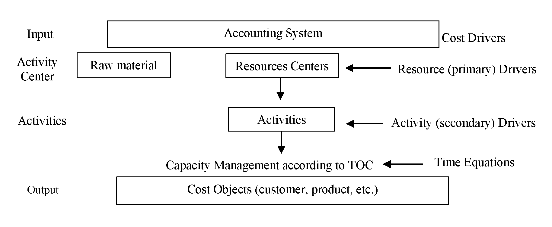
Source: Adapted from Huang et al. (2014).

In a study by Huang et al. (2014) on TDABC and TOC integration, it is focused on the understanding of the production process of the enterprise and the cost structure of the products, and the production process activities and activity centers were also examined within the TDABC system. The maximum capacity of each resource center was determined as theoretical capacity. Subsequently, the capacity requirements of each of the products produced in these resource centers were determined using the time equations regarding these products and compared with the theoretical capacity of the resource centers. As a result of this comparison, if the theoretical capacity of the resource center was found to be below the capacity necessary for the manufacturing of the products in that particular resource center, it may be asserted that a bottleneck is formed in the relevant resource center. From this point forth, within the framework of TOC's five-step continuous improvement approach, ways to eliminate the capacity constraint of the enterprise should be explored. TOC offers five steps in managing constraints: identifying the system constraints, exploiting the system constraints, subordinating other activities in the process, elevating the system constraints, and making the TOC a continuous process (Grida & Zeid, 2019). Zhang & Yi (2008), who applied one of the studies treating the integration of TDABC and TOC systems to examine logistic costs, maintained that both theories gained favor in optimizing business processes and directing activities where capacity utilization was insufficient by the combination of their strengths. Zang & Yi (2008) studied only the logistics process in their case study. Beyond that, the same methodology can be applied as a case study to an entire business, rather than focusing on a particular activity (Santana & Afonso, 2015).

3. Methods

In this study, the case study method was used. The case study method was preferred because it provided a detailed examination regarding a single phenomenon. The case study scientifically investigates a real-life situation in-depth and in its natural setting (Ridder, 2017). The case study method was preferred because it provides the possibility to directly observe the activities to determine the activities that form the production stages one by one and to create time equations based on each product. In the company, where the case study was conducted, the data were obtained through interviews conducted with business executives and employees and by observing production processes.

This study aims to develop solutions appropriate for the five-stage improvement process of TOC to improve capacity constraints and guide management decisions, based on the fact that in a production enterprise manufacturing products with different production stages, the actual capacity utilization determined by using the time equation of TDABC is compared with practical capacity. The capacity usage amounts necessary for the manufacturing of products in a pickle production company operating in Turkey were evaluated with the TDABC system, and TOC was utilized in the identification of the possible constraints in the company with the ways to improve them. Figure 2 shows the application model of TOC and the TDABC system.

Figure 2.

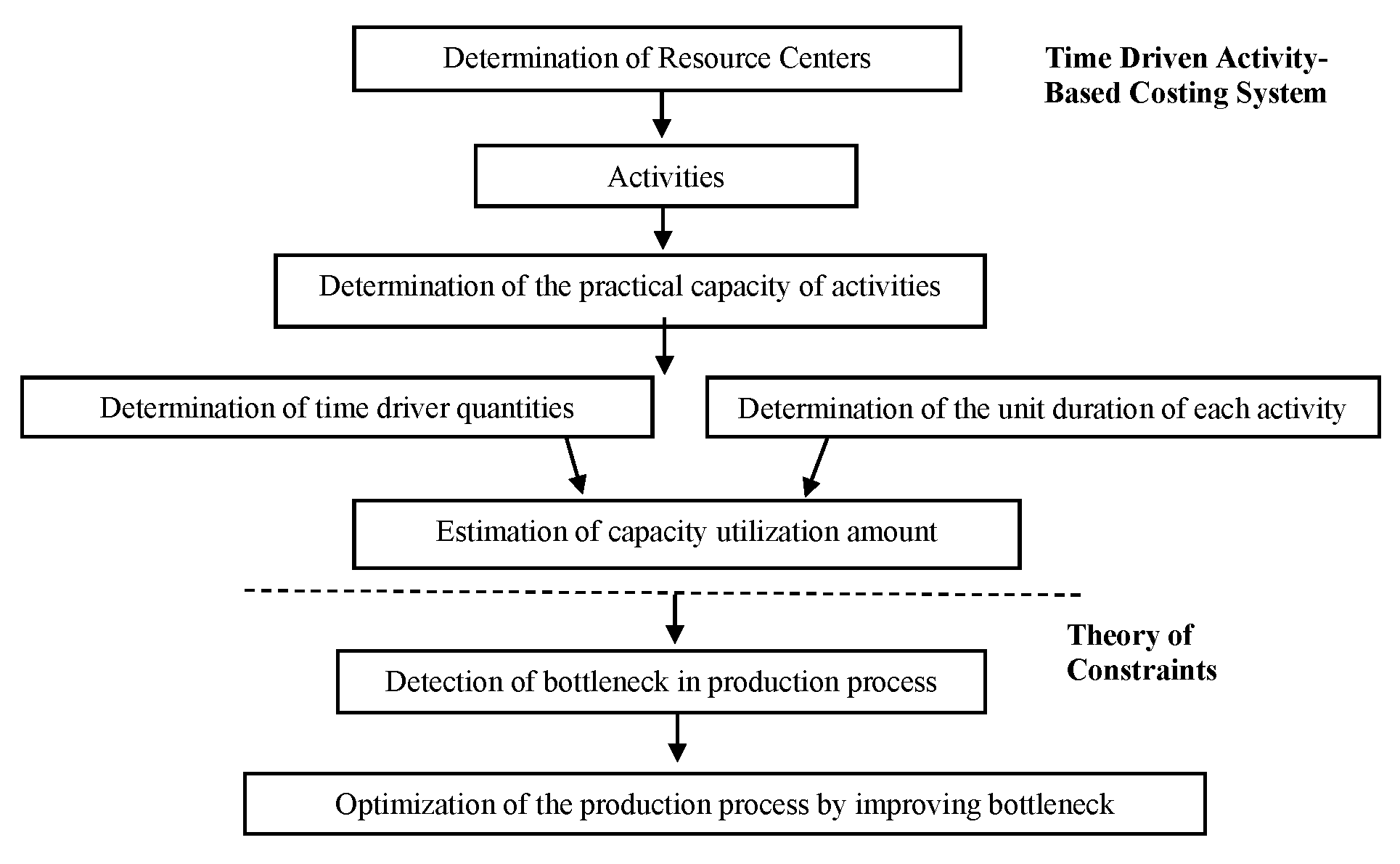
In Figure 2, the model in which TOC and TDABC systems are integrated, the capacity required by the production activities for the manufacturing of the product amount required in the relevant period with time equations is determined. This capacity requirement serves as a constraint function and is represented by T_i. According to the model, if the theoretical capacity of production activities is less than T_i, it may be asserted that there is a capacity constraint (bottleneck) in the production activity concerned (Huang et al., 2014). However, the theoretical capacity cannot be reached as it is not possible to make the employees work during breaks machine maintenance due to legal obligations. Therefore, in this study, actual capacity and practical capacity will be compared instead of theoretical capacity. If

\[ \textit{Practical capacity} < \textit{Actual capacity there is a constraint}. \]

TOC should be guided not only in identifying bottlenecks but also in improving operational processes. Solutions aimed at the elimination of constraints are developed with a five-stage improvement process.

The following stages were applied in the application of TDABC and TOC (Oker & Adiguzel, 2016; Reynolds et al., 2018; Yun et al., 2016; Huang et al., 2014; Zhang & Yi, 2008; Etemadi, 2018; Santana & Afonso, 2015; Ganorkar et al., 2018; Watson et al., 2007):

• The resource centers are identified according to the functions of the activities carried out in the production process of the company.

• Practical capacity has been calculated by deducting the times that caused interruptions in production because of breaks, absenteeism, planned maintenance, and repair hours from the theoretical capacity. The capacity is measured in terms of labor time (minutes).

• Time equations have been formed for each activity.

• The amount of capacity required to produce all products which have been determined using time equations. Then, the actual capacity has been identified.

• By comparing the actual capacity with the practical capacity, it has been evaluated whether there is a bottleneck and idle capacity in the activities in the production process.

• Considering TDABC and TOC together, the results are analyzed and solutions are proposed to determine the most profitable product mix decision with the available capacity and capacity improvements.

4. Results

Three products, pepper pickle, jalapeno, and mixed pickle were discussed. Since vegetables, which are the raw materials of pickles, are collected from the field in summer, the company makes production in summer. The case study was performed on pickled pepper, jalapeno, and mixed peppers, the production of which was conducted in the periods of T₁, T_2, and T₃, respectively. Because the fermentation period required for pickling varies from product to product. Sales are made to both domestic and international retails with 64 personnel in total. Due to confidentiality, the case study company will be represented as ABC Company, and the products examined will be represented as Product X, Product Y, and Product Z.

Pickle production is carried out in two basic stages the brining of pickles and the packaging of pickles. The activity of brine starts with the acceptance of the raw material. The raw material is brought to the company and the cleaning, cutting and washing of the vegetables subject to pickle production according to the type of pickle to be produced are carried out at this stage. The vegetables prepared are preserved as brine in the tanks. All the inputs of the pickle are preserved in the tanks to be fermented at this stage. After the vegetables are fermented and pickled, the tanks are emptied and the products are weighed. The fermentation period varies between products. The fermentation period of X is 30 days and this period is expressed as T₁; the fermentation period of Y is 30 days and this period is expressed as T₂; the fermentation period of Z is 45 days and this period is expressed as T₃ in the study. The vegetables are taken to the pickle packing area after their fermentation process is completed. Pickles taken to the packaging area are chopped, extracted and washed. At this stage, the products are mixed according to the type of pickle. The unwanted parts such as the leaf and stem are again processed through picking and the pickle filling stage begins. In the following process, the vegetable part of the pickle is filled into clean packages and weighed. The final brine is added to these packages and their lids are closed. After the brine is added, the packages are washed and cleaned. In the final stage, the cleaned packages are labeled and made ready for shipment to the finished goods warehouse. In Table 2, various sub-activities are carried out in each activity flow in the two main production stages of the company, which are the brining of pickle and packaging. Table 2 shows all the activities in the pickle production process and the activities carried out in the manufacturing of products X, Y, and Z. Also, resource centers created by dividing activities and sub-activities according to their functions are shown.

Table 2. ABC Company Resource Centers

Resource Centers		Activities		Subactivities	X	Y	Z
Brining of Pickle	A1	Raw Materials and supplies admission	S1	Raw material admission	+	+	+
	A2	Preparation of Vegetables	S2	Drilling	-	+	-
			S3	Leaf separation	+	-	+
			S4	Stem cutting	-	-	+
			S5	Destoning	-	-	+
			S6	Selection extraction	+	+	+
			S7	Cutting	-	-	+
			S8	Transferring of vegetables into tanks	+	+	+
	A3	Brine	S9	Brine preparation	+	+	+
			S10	Pouring the brine into the tanks	+	+	+
			S11	Unloading the tank	+	+	+
			S12	Weighing the product	+	+	+
Pickle Packaging	A4	Preparation of Pickle for Production	S13	Retention in dilution tanks	-	-	+
			S14	Selection extraction	+	+	+
			S15	Chopping	-	+	+
			S16	Tape laying	-	+	+
			S17	Washing	+	+	+
	A5	Mixing in the drum	S18	Mixing in the drum	-	-	+
	A6	Selection Band	S19	Selection band	+	+	-
	A7	Package Filling	S20	Jerky package filling	+	+	-
			S21	Package manual filling	-	-	+
	A8	Weighing	S22	Weighing according to proportions	-	-	+
			S23	Weighing product weight	+	+	+
	A9	Packaging	S24	Last brine preparation	+	+	+
			S25	Brine filling	+	+	+
			S26	Capping	+	+	+
			S27	Package washing-drying	+	+	+
			S28	Metal detector	+	+	+
	A10	Labeling	S29	Printing labels on products	+	+	+

Source: Authors’ own research.

A total of 38 workers work at the ABC Company's pickle brining and packaging stages. 11 of these workers take part in the pickle brining phase and 27 of them work in the pickle packaging phase. In the pickle brining phase, three activities are carried out with 11 workers; raw material acceptance activity, preparation, and the pickling of vegetables. The labor distribution of the activities of this phase is as follows: vegetables, which are the raw materials of pickles, are only delivered to the company in the mornings. For this reason, 11 workers are involved in the transportation of vegetables from trucks to the factory for three hours each morning. In the afternoons, 4 of the same workers perform the preparation activities for vegetables and 7 of them perform the activity of the pickling of vegetables. When evaluated considering this distinction, the number of workers in the company is 38. The workers work 26 days a month and 9 hours a day. However, production is interrupted for various reasons in the company. Due to the periods spent with the maintenance and repair of the equipment used in production, the company cannot reach the 9-hour daily employment period. When these deductions and breaks are deducted from the 9-hour working period, the networking period of the employees is found and as a result of the multiplication of this period with the number of workers, the monthly practical capacity is calculated as 6.072 hours. However, regarding the 3,5 months (30 days+30 days+45 days) encompassing the T₁-T₂-T₃ periods, the total number of practical direct labor hours is 21,250. These calculations are shown in Table 3.

Table 3. Determination of the Number of Direct Labor and Practical Labor Hours in the Activities

Activities		a	b	c	d=a*b*c*	e=d*3,5	f	g	h=d-f-g	i=a*c*h	j=i*3,5
Brining of pickle	A1	11	3	26	858	3.003	0,25	-	2,75	787	2.753
	A2	4	6	26	624	2.184	1,25	2,08	2,67	278	972
	A3	7	6	26	1.092	3.822	1,25	1,56	3,19	581	2.032
Pickle packaging	A4	3	9	26	702	819	1,5	3,12	4,38	342	1.196
	A5	1	9	26	234	4.095	1,5	0,52	6,98	181	635
	A6	5	9	26	1.170	4.095	1,5	0,52	6,98	907	3.176
	A7	5	9	26	1.170	1.638	1,5	1,04	6,46	840	2.939
	A8	2	9	26	468	3.276	1,5	0,52	6,98	363	1.270
	A9	4	9	26	936	5.733	1,5	1,56	5,94	618	2.162
	A10	7	9	26	1.638	819	1,5	1,04	6,46	1.176	4.115
	Total				8.892	31.122				6.072	21.250
a: Number of direct workers b: Hour c: Day d: Monthly theoretical direct labor hours				e: Total theoretical direct labor hours f: Break time g: Scheduled maintenance and repair time *T1-T2-T3 periods were 3.5 months.					h: Net working hours i: Monthly practical direct labor hours j: Total practical direct labor hours

Source: Authors’ calculation

Time estimates of activities are made through time equations. Time equations were calculated based on the following formula (1).

\[\begin{equation} \label{eq1} \small t_{j,\ k} = \beta_{0} + \beta_{1}X_{1} + \beta_{2}X_{2} + \beta_{3}X_{3} +... + \beta_{P}X_{P} \ \ \ \ (1) \end{equation}\]

These parameters (Santana & Afonso 2015):

• \(t_{j,\ k}\) = time required to execute event k of activity j

• \(\beta_{0}\) = fixed time for activity j, independent of the characteristic property of event k

• Time spent for one unit of time factor 1 while \(\beta_{1} = X_{2}, X_{2},..., X_{PA}\) is constant

• \(X_{1}\) = time factor 1

• P = number of time factors used to determine the time needed for the j activity carried out

Table 4 includes the quality and quantity of time drivers regarding the activities. The periods and amounts of the utilization of each activity are effective in determining the actual capacity of the products. Multiplying the unit of time of the activity by the time drivers showing the amount of the product utilization from the activity shows the capacity needed for the manufacturing of the product. The duration of use of the activity for the product is determined based on time equations. For example, for the A2 activity in the production of X Product, the following time equation was formed and calculated and time equations were formed in the same way for the other activities.

A2 = (0,12 * X1) + (0,12 * X1) + (0,027 * X1) + X1: Amount given to production

In this context, the capacity amounts used in the production of X, Y and Z products are shown in Table 4.

Table 4. Determination of the Actual Capacity Used in Manufacturing Products

A1-10	S1-29	Quality of time drivers (kg)	Product X	Product Y	Product Z
			Amount of time drivers (kg) * Unit of time (min.) = Total Actual Capacity
A1	S1	Amount of incoming raw materials	520.000 * 0.015 = 7.800	520.000 * 0,02 = 7.800	540.020 * 0,02 = 8.100
A2	S2	Amount given to production	-	260.000 * 0,06 = 15.600	-
	S3		260.000 * 0,120 = 31.200		2.600 * 0,12 = 312
	S4		-	-	2.600 * 0,12 = 312
	S5		-	-	2.600 * 0,12 = 312
	S6		260.000 * 0,120 = 31.200	260.000 * 0,12 = 31.200	260.000 * 0,12 = 31.200
	S7		-	-	104.000 * 0,03 = 3.566
	S8		260.000 * 0,027 = 6.933	260.000 * 0,03 = 6.933	260.000 * 0,03 = 6.933
A3	S9	The amount of input in brine	88.400 * 0,005 = 398	132.600 * 0,005 = 597	135.200 * 0,005 = 608
	S10		88.400 * 0,005 = 398	132.600 * 0,005 = 597	135.200 * 0,005 = 608
	S11		88.400 * 0,024 = 2.122	132.600 * 0,02 = 3.182	135.200 * 0,02 = 3.245
	S12		88.400 * 0,033 = 2.947	132.600 * 0,03 = 4.420	135.200 * 0,03 = 4.507
A4	S13	Amount given to production	-	-	103.584 * 0,80 = 82.868
	S14		145.600 * 0,004 = 582	145.600 * 0,004 = 582	103.584 * 0,004 = 414
	S15		-	145.600 * 0,05 = 7.280	103.584 * 0,05 = 5.179
	S16		-	145.600 * 0,02 = 2.184	103.584 * 0,02 = 1.554
	S17		145.600 * 0,005 = 728	145.600 * 0,01 = 728	103.584 * 0,01 = 518
A5	S18	Incoming amount	-	-	103.792 * 0,01 = 1.038
A6	S19	Incoming amount	145.600 * 0,057 = 8.320	145.600 * 0,06 = 8.320	-
A7	S20	Incoming amount	145.600 * 0,057 = 8.320	145.600 * 0,06 = 8.320	-
	S21		-	-	103.792 * 0,09 = 8.896
A8	S22	Amount produced	-	-	103.792 * 0,12 = 12.455
	S23		145.600 * 0,054 = 7.804	145.600 * 0,003 = 7.804	103.792 * 0,05 = 5.563
A9	S24	Amount produced	145.600 * 0,030 = 4.368	145.600 * 0,03 = 4.368	103.792 * 0,03 = 3.114
	S25		145.600 * 0,061 = 8.885	145.600 * 0,06 = 8.885	103.792 * 0,06 = 6.334
	S26		145.600 * 0,061 = 8.885	145.600 * 0,06 = 8.885	103.792 * 0,06 = 6.334
	S27		145.600 * 0,061 = 8.885	145.600 * 0,06 = 8.885	103.792 * 0,06 = 6.334
	S28		145.600 * 0,061 = 8.885	145.600 * 0,06 = 8.885	103.792 * 0,06 = 6.334
A10	S29	Amount produced	170.170 * 0,040 = 6.807	170.170 * 0,04 = 6.807	176.436 * 0,04 = 7.057
		Total	155.466	152.261	213.693

Source: Authors’ calculation

The raw materials of the Z product are only processed through pepper and capia pepper leaf separation, stem cutting and seed extraction. Since these vegetables form 10% of the product, the time driver amount of the related activities are regulated accordingly. According to Table 4, Z uses most of the capacity for its production.

In the model in which TOC and TDABC systems are integrated, the capacity required by the production activities for the manufacturing of the product amount requested in the relevant period with time equations is determined. This capacity requirement serves as a constraint function and is expressed as T_i. According to the research model, if the practical capacity of production activities is less than the capacity required for the manufacturing of products, it can be said that there is a capacity constraint (bottleneck) in that production activity. TOC should be guiding not only in identifying bottlenecks but also in improving operational processes. Solutions aimed at the elimination of constraints are developed with a five-stage improvement process. In this context, Table 5 presents the amount of time required for the manufacturing of product X, product Y and product Z, and its distribution according to the activities and products as calculated by the time equations.

Table 5. Total Capacity Requirement of Products According to Time Equations

Activities	Product X (min.)	Product Y (min.)	Product Z (min.)	Total
A1	7.800	7.800	8.100	23.700
A2	69.333	53.733	42.635	165.702
A3	5.864	8.796	8.968	23.628
A4	1.310	10.774	90.533	102.618
A5	-	-	1.038	1.038
A6	8.320	8.320	-	16.640
A7	8.320	8.320	8.896	25.536
A8	7.804	7.804	18.018	33.627
A9	39.907	39.907	28.448	108.268
A10	6.807	6.807	7.057	20.671
Total	155.466	152.261	213.693	521.421

Source: Authors’ calculation.

Table 6 shows the bottleneck activity periods identified. For this, the practical capacity of the activities and the capacity required for the production of the products were compared. The total practical capacity of the activities is shown in the form of the data in Table 3 converted to minutes and the capacity required for the production of the products is conveyed from Table 5.

Table 6. Detection of Bottleneck in Activities

Activities	Practical Capacity (min.)	Required Capacity (min.)	Difference
A1	165.165	23.700	141.465
A2	58.313	165.702	-107.389
A3	121.922	23.628	98.294
A4	71.744	102.618	-30.873
A5	38.111	1.038	37.073
A6	190.554	16.640	173.914
A7	176.358	25.536	150.822
A8	76.222	33.627	42.595
A9	129.730	108.262	21.468
A10	246.901	20.671	226.230
Total	1.275.019	521.421	753.598

Source: Authors’ calculation.

According to the research model, if the total capacity required by the activity for the manufacturing of the products is more than the practical capacity of the activity, it is said that there is a bottleneck in that activity. The production activities of the ABC Company are evaluated and "A2" and “A4” activities comprise capacity constraints. While the total practical capacity of A2 activity is 58.313 minutes, the time required to produce these products is 165.702 minutes. Since the capacity requirement of the activity is 107.389 minutes longer than its practical capacity, the bottleneck is identified in the activity. Similarly, while the total practical capacity of the A4 activity is 71.744 minutes, the time required to manufacture the products is 102.618 minutes. Since the capacity requirement of the activity is 30.873 minutes longer than its practical capacity, the bottleneck is also identified in this activity.

5. Discussions

As a result of the implementation of TOC used together with the TDABC system, in the company subject to the application, answers to the questions of whether it provides benefit to the management in process and cost improvement were sought. According to Goldratt & Cox (2016), in the case of a bottleneck, there are two ways to remedy the bottleneck: the first is to avoid wasting time in the bottleneck, and the second is to explore ways to increase the bottleneck capacity. TOC provides various solutions for the elimination of constraints. A five-step improvement process is used to manage constraints and to continuously improve business processes (Ruhl, 1996). Below are suggestions for eliminating bottlenecks within the framework of the “Five-Stage Improvement Process” of TOC.

Stage 1 Determining the constraints of the system: When the capacity calculations required for production in ABC Company were evaluated with the practical capacity of the activities of the company, it was found that A2 and A4 activities do not meet the capacity required for production. In this respect, a capacity constraint is seen in A2 and A4 activities.

Stage 2 Deciding how to resolve the constraints in the system: At this stage, the optimal product mix is determined when there is a constraint. In the case of limited production resources in a company, the product mix should be determined (Sobreiro et al., 2014). Since there are two constraints in the system, a linear programming model is utilized to determine the optimal product mix. The throughput of the products is taken into consideration in determining the optimal product mix. Table 7 shows the calculation of throughput for each product.

Table 7. Determination of Throughput of Products

(in kg)	X	Y	Z
Sale Price (a)	5,14	4,8	2,62
Direct material costs (b)	2.63	1.91	1.23
Throughput (c) = (a-b)	2.51	2.89	1.39

Source: Authors’ calculation

When their throughput is considered, the production of X and Y should be given priority. The model for the optimal product mix is shown in function 2 and function 3 (Sobreiro et al., 2014):

\[\begin{equation} \label{eq2} \small \text{Max. Z} = \sum_{i = l}^{n}{(\text{p}_{i} –\ \text{c}_{i})\ \text{q}_{i}} \ \ \ \ (2) \end{equation}\]

\[\begin{equation} \label{eq3} \small \begin{split} &\sum_{i = l}^{n}{(\text{a}_{ij},\ \text{q}_{i})\ \leq \ R_{j} } \ \ \ \ (3)\\ &\text{q}_{1} \leq \text{d}_{I}; j = 1, 2,..., m; i = 1, 2,..., n \end{split} \end{equation}\]

j = 1, 2,…, m number of products

i = 1, 2,…, n number of resources

p_i selling price of the i product

c_i the cost of the i product

a_ij amount of source j required to manufacture product i

R_j the maximum amount of source j available

q_i production quantity of i product

d_i quantity of product i requested

In the linear programming model created for TOC, the value to be maximized in the objective function is calculated by simply subtracting the cost of the direct materials from the sales price of the products (Demirciolu & Demirciolu, 2016). These values are calculated in Table 7 and are shown in the following objective function 4. Capacity constraints regarding A2 and A4 activities are shown in equations 5 and 6, and restrictions on the quantity of demand for products are shown in equations 7, 8, and 9.

\[\begin{equation} \label{eq4} \small \text{Max. Z} = 2.51 X + 2.89 Y + 1.39 Z \ \ \ \ (4) \end{equation}\]

Constraints: \[\begin{equation} \label{eq5} \small A2: 0.267 X + 0.21 Y + 0.54 Z \leq 58.313 \ \ \ \ (5) \end{equation}\] \[\begin{equation} \label{eq6} \small A4: 0.009 X + 0.084 Y + 0.884 Z \leq 71.744 \ \ \ \ (6) \end{equation}\] \[\begin{equation} \label{eq7} \small X \leq 182,000 \ \ \ \ (7) \end{equation}\] \[\begin{equation} \label{eq8} \small Y \leq 273,000 \ \ \ \ (8) \end{equation}\] \[\begin{equation} \label{eq9} \small Z \leq 159.120 \ \ \ \ (9) \end{equation}\]

A2 and A4 have constrained activities, and the periods required to produce a unit of X, Y, and Z products are shown in the model in such a way that they do not exceed the total capacity of the activities. The product mix that will provide maximum throughput with the linear programming model is shown in Table 8.

Table 8. Determination of Optimal Product Mix

	X	Y	Z	Total		Right Side
A2	0,267	0.21	0.54	58.313	≤	58.313
A4	0,009	0,084	0,884	22.965,13	≤	71.744
Demand of X	1	0	0	3.681,648	≤	182.000
Demand of Y	0	1	0	273.000	≤	273.000
Demand of Z	0	0	1	0	≤	159.120
Purpose F.	2.51	2.89	1.39
Decision D.	3.681,648	273.000	0
Max Z.	798.210,9

Source: Authors’ calculation

As a result of the solving of the linear programming model in MS Office Excel, the whole Y product is 273.000 kg. and 3.682 kg of production should be made from X product. As a result, the expected throughput is 798,211.

Stage 3 Subordinating the whole system to eliminate the constraint: At this stage, other resources should be planned in accordance with the decision regarding the product mix made in the second stage.

Stage 4 Deciding to eliminate the constraint: This is the stage in which solutions involving long-term investment decisions are applied to eliminate the constraint. The capacity constraint seen in A2 and A4 activities was the result of the inability of the existing capacity to meet production. A2 activity is the process in which the products are prepared for brine and prepared for storage in tanks for fermentation. These activities are the production stages in which both labor and machine use take place. In A2 activity, 107.389 minutes of missing capacity was detected. In the A4 activity, 30.873 minutes of missing capacity was calculated. Therefore, the following alternative suggestions have been made to remedy this situation:

• To generate new employment or to provide overwork so that the constraint in bottleneck activities is eliminated:

  • A2 Preparation of vegetables: The capacity required to meet the total production is 165.702 minutes. The current capacity is 58.320 minutes. Accordingly, the missing capacity is 107.382 minutes. In this case, the effect of solutions on capacity is shown in Table 9:

Table 9. Effect of Overwork and Additional Employment on A2 & A4 Capacity

	Employee	Hour	T1-T2-T3 Total Days	Total Hours	Total Minutes
A2 Capacity
Available	4	2,67	91	972	58.320
Overwork	11	2	91	2.002	120.120
Additional Employment	3	7,5	91	2.407	122.850
A4 Capacity
Available	3	4,38	91	1.196	71.760
Overwork	3	2	91	546	32.760

Source: Authors’ calculation.

If 4 people work full time, the bottleneck is solved, but these workers are also used in other jobs. According to this, either the workers perform 2 hours of extra work, or if they are to work in a single shift, 3 additional workers are employed in the summer period, even if it is temporarily. In Table 9, as a result of overwork practice, the total capacity reaches 178.440 (58.320 + 120.120) minutes. As a result of overwork practice, the total capacity reaches 181.170 (58.320 + 122.850) minutes. As a result of both solutions, the capacity required for production is more than 165.702 minutes.

• A4 Preparation of the pickle for production: The capacity necessary to meet the total production amount is 102.618 minutes. As a result of this application, the capacity is expected to be as follows. With the practice of overwork, the activity will reach 104.520 (71.760 + 32.760) minutes and it is expected that the capacity constraint is eliminated in Table 9.

Stage 5 System recurrence: This stage refers to a return to the first stage for the detection of another constraint after the constraint in the system has been eliminated. After the capacity constraint has been eliminated, the production quantities will be adapted to this situation in the long run, and thereafter the company will possibly face a market constraint. It should be returned to the first stage for the recurrence of a bottleneck to be prevented.

The capacity constraint in the company was determined by evaluating in terms of TOC. Suggestions have been developed for the constraints within the framework of the TOC Five-Stage Process Improvement method. Therefore, the TDABC system was treated together with TOC in the ABC Company and solutions regarding constraints could be proposed. As a result, the company has provided a perspective in terms of throughput to the product cost by treating the TDABC and TOC systems together, and different solutions were offered regarding the determination and elimination of capacity constraints.

6. Conclusions

The main point of view regarding the joint application of TOC and TDABC systems guides business managers in determining efficient and inefficient activities and detecting idle capacity. The TDABC system provides useful information for capacity management. TOC, on the other hand, is a management philosophy. It is not interested in determining costs but focuses on eliminating all the factors that reduce profit in a system. The TOC approach includes different methods for managing constraints. Using these methods, solution offers are developed to eliminate the constraints that reduce the profitability and performance of the company. In summary, the TDABC system sheds light on production decisions based on the extent of benefiting from activities, determination of the unnecessary time consumed by the activities and the idle capacity. TOC, which is also a management accounting approach, is a multi-faceted approach that aims to improve all kinds of factors that prevent a company from increasing its profit and performance and to offer and apply new approaches and solutions to business management.

The main purpose of this research is to determine the use of capacity with the TDABC system and to investigate the possible capacity, process and cost improvements according to the TOC approach, which serves as a guideline in increasing operational performance. The capacity utilization amounts of the products were calculated by using the time equations of the TDABC system. From this point forth, these results were evaluated within the scope of TOC, the capacity utilization amounts required for the manufacturing of the products were compared with the existing capacity of the resource centers and potential capacity constraints in the production activities were determined. In the following stage, how the capacity constraints determined by the five-step process improvement method, which is the guiding method regarding TOC's constraint management was shown with the case study in the research. The following conclusions were reached in the research:

• 10 activities consisting of many sub-activities were identified. When the practical capacity of these resource centers and the actual capacities of TDABC determined with the help of time equations were compared, it was determined that the capacity to meet the orders received during the research period was not available. In this respect, A2 and A4 were identified as bottleneck resources in the company.

• The five-stage continuous improvement model of TOC was applied to improve bottleneck resources. As a result of this application, short term and long-term solutions were developed:

  • The optimal product mix was determined by utilizing linear programming for maximum profitability in the short term. Accordingly, the most profitable product mix was created according to throughput accounting and it was concluded that product Z should not be produced.

  • In the long run, overwork with the existing workforce or the employment of three additional employees to overcome capacity constraints were offered as a solution to increase the capacity of bottleneck resources.

• In other activities, the presence of idle capacity was determined. For this purpose, it was observed that the company should have the appropriate quality certificate to be able to work with larger retailers.

With this implementation, it has been observed that the TDABC system and TOC approach can work together in determining the throughput, constraints and managing the capacity constraints in a production company. As a result of the literature research, TOC was generally examined together with the ABC system, which is one of the contemporary management accounting systems, and applied in the TOC product mix decisions in the determination of product costs by ABC systems. But in this study, the capacity required for the manufacturing of products was determined within the framework of the TDABC system while the principles of TOC were evaluated in terms of capacity management. It is thought that the study will contribute to the literature as it is based on practical capacity in determining idle and bottleneck capacity, takes into account all activities of the enterprise in time-oriented activity analysis and that TDABC supports product mix decisions within the framework of TOC. The practical implications of the study are an implementation of the TDABC system and the TOC approach together in businesses that produce different products and where each product goes through a production process that includes different activities. It can be said that the results of the study help to guide the managerial decisions such as product mix decisions, order acceptance or rejection decisions, overwork, new staff recruitment decisions by utilizing linear programming regarding the elimination of the bottleneck in companies and thus to improve the profitability and efficiency of the companies.

The limitations of the study can be listed as follows: Due to the nature of the case study, the result of these findings cannot be generalized. The diversity of production activities in the company, interviews with engineers and managers took time to determine the activity periods. Since the vegetables, which are the raw materials of pickles, were brought to the factory from the field mostly during the summer months, the study was conducted only in a period limited to the summer season. For further research, the TDABC system can be applied not only to production enterprises in different sectors but also to service businesses. The period of the application can be expanded. Data can be created for the food industry by applying to different food businesses.