The Impact of Mayors’ Corruption on Spanish Municipal Spending
ABSTRACT
We investigate the impact of mayors’ corruption on the size and structure of Spanish municipal budgets. The theory posits that total expenditure is greater in corrupt governments: €77.08 higher per capita in our sample when a corrupt mayor is in office. Moreover, the literature predicts that mayors (agents), will spend more on items directly connected with corruption, rather than expenditure priorities demanded by the citizens (principals). Thus, we show that total expenditure, capital, trash collection and police are higher when corruption exists. Literature predicts that corrupt mayors spend less on items that provide fewer opportunities to collect bribes: our data show that corrupt mayors do not spend more on health. Corrupt mayors spend on average 1.46 years on duty after being taken to court with a formal indictment on a corruption charge. This indicates that in Spain, sadly, resigning the mayoralty is not automatic when facing criminal charges for corruption.
Keywords: Corruption, Mayor, Municipal expenditure.
JEL classification: D73, H20, H71.
El impacto de la corrupción de los alcaldes en el gasto municipal español
RESUMEN
Investigamos el impacto de la corrupción de los alcaldes en el tamaño y la estructura de los presupuestos municipales españoles. La teoría postula que el gasto total es mayor en los gobiernos corruptos: 77,08 euros más per cápita en nuestra muestra cuando un alcalde corrupto está en el cargo. Además, la literatura predice que los alcaldes (agentes), gastarán más en partidas directamente relacionadas con la corrupción, en lugar de en los gastos demandados por los ciudadanos (principales). Así, mostramos que el gasto total, el gasto de capital, la recogida de basura y la policía son mayores cuando existe corrupción. La literatura predice que los alcaldes corruptos gastan menos en partidas que ofrecen menos oportunidades de sobornos: en este sentido, nuestros datos muestran que los alcaldes corruptos no gastan más en sanidad. Los alcaldes corruptos están una media de 1,46 años en activo tras ser llevados a juicio con una acusación formal por corrupción. Esto indica que en España, lamentablemente, renunciar a la alcaldía no es automático cuando se enfrenta a cargos penales por corrupción.
Palabras clave: Corruption, Mayor, Municipal expenditure.
Códigos JEL: D73, H20, H71.
1. Introduction
This paper investigates the role mayors’ corruption plays in determining municipal budgets. While the literature has focused mainly on the impact of corruption on the global economy, few studies have investigated its impact on municipal budgets. The high level of corruption in the public sector in Spain, and particularly in municipalities, makes our sample suitable for our aim. Thus, this article presents the first research on the impact of mayors’ corruption on Spanish municipal budgets through a comprehensive panel data for the 145 Spanish municipalities over 50,000 inhabitants from 2002 to 2013.
Mauro (1995) acknowledges that corruption would be beneficial for citizens (principals) as a way to encourage government employees to work harder and this way overcome the excessive bureaucracy (red tape). However, the corruption considered in this article is negative for taxpayers, since it just means private illegal gain for the mayor. Besides, the red tape in Spain, although it exists, does not prevent normal economic and business development.
Empirical evidence shows that bribes can be collected more efficiently on some government expenditure components than on others (Mauro, 1996). Accordingly, this article studies several expenditure items that the literature has identified as being connected with corruption.
Our assumptions state that corrupt mayors impact municipal budgets in three ways (Liu & Mikesell, 2014). First, increasing total expenditure per capita. Second, changing budgets towards corrupt-related expenditure items. Third, decreasing budget expenditures in those items that do not allow corruption.
The paper is organized as follows. First, electoral impact of corruption is described. Next, we explain the links between corruption and government budgets. Then, we present our econometric model, results and discussion. Finally, we summarize our conclusions and indicate policy implications.
2. Electoral implications of corruption
In Max Weber’s ideal bureaucracies, the public official (agent) is the faithful executor of the mandate and instructions that he receives from the state (principal). In this Weberian public sector, no principal-agent problems would develop. Unfortunately, in real world, Weberian bureaucracies are rare (Tanzi, 1998). The agency theory posits that the agent is better informed than the principal, in a political setting in which voters, as principals, elect politicians who, as agents, make policy choices that affect voters. The agency theory shows that the interests of agents and principals are not aligned, thus, mayors may maximize budgets for their own private gain. Electoral competition should be an effective solution to principal-agent problem among politicians and voters (Wittman, 1989). As Montinola & Jackman (2002) and Benito (2016) point out, one mechanism through which political competition reduces corruption is the re-election imperative, which lowers the demand for bribes. Political competition is posited to reduce corruption in two additional ways (Montinola & Jackman, 2002; Benito, 2016). First, the freedom of information and association characteristic of democracies helps monitoring public officials, thereby limiting their chances of corrupt behavior. Chang et al. (2010) state that a vigilant and free press is essential for political accountability in democracies, since an independent judiciary is not a sufficient condition to help voters curb corruption. This freedom of information helped build our corruption variable, as we will describe later. Second, the possible turnover of power in democracies implies that policies may be reversed by future politicians, thus incumbents in power cannot always promise that particular laws will continue in the future. This minimizes the size of bribes that rent-seekers are willing to pay (Chang et al., 2010).
However, some authors such as Wagner et al. (2009) and Ríos et al. (2017) argue that if politicians cannot be trusted due to corruption, then citizens may decide not to participate and may abstain in the coming elections. Accordingly, for elections to be an efficient monitoring mechanism, mayors charged with corruption should be punished by proactive voters in the coming election, in the case that they do not resign immediately after being charged. In our data, mayors spend, on average, 1.46 years on duty after being accused. This indicates a failure in the Spanish political framework, as predicted by Wagner et al. (2009), inasmuch as mayors do not feel the pressure to resign, a pressure that public opinion would exert in other countries.
3. Corruption and government budget
Measuring the effects of corruption on government expenditure may help assess the principal-agent problem between citizens and politicians (Mauro, 1998). In fact, some authors consider corruption as a behavior of public officials that deviates from principal-agent agreements that exist in democracy between voters, politicians, and bureaucrats (Lancaster & Montinola, 2001). One of the explanations found by Tarschys (1975) for government expenditure growth is the legitimacy of the government. In this respect, if citizens believe that there is a great deal of corruption in government, they will oppose higher expenditures. Relative mistrust of politicians seems to be determinant when it comes to explain the level of public spending.
According to Lowery & Berry (1983), government growth can be the result of either a responsive government or an excessive government. In the former case, governments do not spend more by their own decision, but they just meet citizens’ demand for public services. In the latter, governments themselves determine their size, i.e., they operate to expand government spending beyond the level demanded by the public. There are several models within the excessive government theory. One of these models, the role of bureaucratic self-interest, would explain public sector expansion as a way for “self-interested” politicians to manipulate budgets for their own private gain. This manipulation meets Mauro (1995) definition of corruption: “misuse of public office and authority for private gain”, and it is in line with the corruption variable used in this paper.
Larmour & Wolanin (2013) identify several types of corruption by what it involves: bribery, theft of assets, patronage, cronyism or distortion of government expenditure. We identify corrupt mayors when they are taken to court, and based on that indication of the existence of corruption, we analyse the last type of corruption, i.e., distortion of government expenditure. Seligson (2002) points out several negative effects of corruption. First, public services focus toward those who pay bribes, denying those services to those who do not, thereby resulting in uneven and often inferior services to many. Second, bribes enable government contractors to avoid legal requirements and offer substandard goods or services (e.g., roads that deteriorate rapidly). Third, corruption weakens the rule of law and, as a result, it makes transactions irrational from an economic point of view (e.g., contracts are not awarded to the highest quality, lowest cost bidder, but to the firm that pays the highest bribe). By increasing expenditure per capita, public services are costlier than the economic optimum, as a way for politicians to get bribes out of the extra cost. This supplementary cost is financed by taxpayers, since municipal budgets must be balanced in Spain. Thus, this funding may be immediate, through higher-than-optimal taxes, or deferred, through higher-than-optimal municipal debt, which creates fiscal illusion. Our empirical results will show that rather than borrowing or taxes, higher grants from upper level governments have partially funded the greater expenditure in corrupt mayors’ municipalities.
The political elasticity theory identifies two types of corruption. Primary corruption indicates excessive partisanship or greed, while secondary corruption indicates the government’s inability to control or mitigate this situation (Werlin, 2003). Therefore, corruption is a balance between greed and governance. The weaker the governance, the more dangerous the manifestations of greed. Because secondary corruption undermines an already weak governmental system, it requires fundamental political reform before punitive measures can be effective. The corruption investigated in this article has to do with primary corruption because it stems from mayors’ greed. As a result of our empirical analysis, some policy implications within the political elasticity theory will be suggested. Thus, though secondary corruption does not exist in Spanish municipalities, political reforms should be implemented to tackle mayors’ corruption. These reforms should enhance municipal governance, so that the balance between greed and governance is dominated by the latter.
4. Impact of corruption on government expenditures
4.1. Total expenditure
Corruption increases public spending, i.e., bribes are considered in the budget calculation. Thus, the budget is a sum of allocated spending plus bribes (Tanzi, 1998). As Rose-Ackerman (1999) points out, not all procurement and contracting scandals involve large-scale construction or capital goods projects, but corruption may involve the whole budget. For example, goods that are consumed are candidates for payoffs because it may be difficult ex post to discover whether or not they were actually delivered. According to Liu & Mikesell (2014), public officials are likely to manipulate government institutions to maximize budgets for their own private gain. Hence, budget of states with a higher degree of corruption will become larger. Rose-Ackerman (1999) shows that corrupt municipalities spend 18 percent more than their non-corrupt counterparts. When countries’ corruption indicators increase, the shares of rent-creating public spending in government budgets also increase, as Hessami (2014) empirically proves. However, Artés et al. (2015), on a sample of Spanish local governments, show that total expenditures decrease by approximately 8 per cent after the corruption scandal is revealed.
Though most of the literature points at larger total expenditure if corruption exists, Mauro (1998) has shown that corruption may have no impact on total government spending. In the same way, Montinola & Jackman (2002) posit that minimizing corruption requires decreasing government intervention in the economy and the number of government officials with discretion over economic activities. These authors find some evidence that the larger the public sector in terms of government expenditures, the lower the incidence of corruption.
4.2. Capital expenditure
Kenny (2007) explains why corruption exists in the construction activity implemented by governments. First, construction involves large, nonstandard activities, so the quality of construction can be very hard to assess. Second, domestic and international construction companies are dominated by a few monopolistic firms. Third, the industry is closely linked to governments, since the latter have major roles as “clients, regulators, and owners” of construction companies. Furthermore, these capital projects normally follow a legal tender. As Gong & Zhou (2015) indicate, formal tendering rules may be modified, circumvented, or replaced by informal ones which facilitate corruption. It is very common to bribe government officials to gain or alter contracts and to circumvent legal requirements. In fact, in Spain, some mayors have joined big construction companies as executives after leaving politics.
Governments with greater levels of corruption tend to invest in housing and physical capital rather than health and education (De la Croix & Delavallade, 2009). In a similar way, Tanzi & Davoodi (1997) and Liu & Mikesell (2014) show that corruption increases public investment projects (construction, infrastructures, etc.) because these projects allow manipulations by high-level officials to get bribes.
One of the reasons why corruption is costly is the distortions stemming from the secrecy of corruption. The demands of secrecy can shift investments away from the highest value projects, such as health and education, into potentially useless projects, such as infrastructure, if the latter offers better opportunities for secret corruption (Shleifer & Vishny, 1993). Tanzi & Davoodi (1997) have tested the hypothesis that higher corruption is associated with higher public investment. Corrupt rulers favor capital-intensive public projects over other types of public expenditures and favor public investment over private investment (Rose-Ackerman, 1999). They will frequently support “white elephant” projects with little value in promoting economic development (Mauro, 1998). Unfortunately, these “white elephant” projects have been common in Spanish municipalities, especially during the years of the “property bubble” (2000-2008), when many municipalities were collecting huge amounts of resources. However, Artés et al. (2015) find that, after the corruption scandal is revealed, investment expenditures decrease since funds are no longer available for construction and infrastructure projects. Currently, most of these facilities remain closed due to the high costs needed to keep them open: sports centers, swimming pools, malls, cultural centers, etc.
Finally, it is important to note that public investment projects may be affected not only by corruption, but also by the existence of political budget cycles. In this sense, Rogoff (1990) and Drazen & Eslava (2010) states that incumbents, before elections, increase the type of spending that is more visible to voters (current spending) and decrease the spending category that is less visible (capital spending).
4.3. Police and wages and salaries
In some cases, leaders use the machinery of government both to enrich themselves and to provide jobs for supporters. A statistical study found that in corrupt cities, wages for lower-skilled workers were 8 percent higher. Besides, corrupt municipalities spent more on general administration and police and fire services, which are areas with many patronage jobs. In Boston, for example, salaries in the city were three times greater than for comparable jobs in the state government and the private sector (Rose-Ackerman, 1999).
According to La Porta et al. (1999), contrary to the view that higher pay for bureaucrats is a remedy for corruption, it is likely instead that powerful bureaucrats collect both higher wages and significant bribes.
Montinola & Jackman (2002) posit that if public officials’ salaries are reasonable, they will value their positions more highly and will have fewer incentives to put those positions at risk by engaging in corrupt behavior. Corruption may also increase when governments are under pressure to reduce the public wage bill’s share in the budget but find it politically difficult to do so (World Bank, 1997). Pay cuts lower resistance to corruption, and if they make it impossible for staff to maintain basic living standards, even the honest can be driven to absenteeism and moonlighting activities that may conflict with their roles as public servants. Finally, Benito et al. (2018) show that higher wages do not reduce politicians’ incentives to engage in corrupt activities.
4.4. Borrowing
Corrupt public officials may have stronger incentives to increase government debt and this way create fiscal illusions that make citizens underestimate their fiscal burdens (Liu & Mikesell, 2014). This behavior leads to higher-than-optimal levels of debt, and it is connected to capital projects such as construction, facilities and highways, since most municipalities fund them through debt. As we said above, these projects offer opportunities to receive rents. Liu, Moldogaziev & Mikesell (2017) show that public corruption is a significant determinant of public debt expansion in America. The levels of public debt issued by state and local governments appear to be higher as corruption increases (Benito et al., 2003).
4.5. Sewer, water and trash collection
Rauch (1995) points at road and sewer investments as eligible to corrupt activities. Similarly, Hessami (2014) posits that there is mounting evidence for corruption connected to expenditures on waste (water) management. However, Rose-Ackerman (1999) shows that in cities where corruption was curbed, they spent proportionately more on infrastructure projects such as roads, waterways, sewers, and water.
4.6. Education
Mauro (1998) points at education as a particularly unattractive target for rent-seekers, presumably in large part because its provision typically does not require inputs to be provided by oligopolistic suppliers. Thus, he finds that corruption alters the composition of government expenditure, specifically by reducing government spending on education. Fisman & Gatti (2002) confirm Mauro (1998) findings, for they identify education spending as one of the activities with low rent extraction potential. Delavallade (2006) and De la Croix & Delavallade (2009) find that corruption impacts negatively the portion of education in government expenditure. Shleifer & Vishny (1993) argue that due to secrecy that surrounds corruption, governments involved in corruption will spend less on education.
4.7. Social protection
According to Mauro (1998), in spending areas such as transfers and welfare payments, many of which constitute rents, bureaucrats sometimes enjoy elbowroom on how to allocate them. For example, bureaucrats may have little room for maneuver on old-age pensions, but, in some countries, fraud is widespread on disability pensions or unemployment benefits. Delavallade (2006) shows that corruption reduces the share of social protection in total spending. Hessami (2014) points out that since social protection represents redistribution between different population groups that is unlikely to be influenced by lobbying firms, the relative importance of this expenditure category decreases with corruption. The reason is that this category provides very few opportunities for rent creation.
4.8. Health
Mauro (1998) finds some evidence that corruption reduces spending on health. Delavallade (2006) shows that corruption reduces the share of health expenditure in total spending. De la Croix & Delavallade (2009) argue that governments with greater levels of corruption tend to invest less in health. Shleifer & Vishny (1993), as we said before, argue that corruption demands secrecy, which is connected with lower investments in health.
Nevertheless, Hessami (2014) finds that a one-unit increase in perceived corruption (on a scale from 0 to 10) is ceteris paribus correlated with an increase in expenditures on health (significant at the 10% level).
5. Empirical Model
5.1. Sample and Variables
The sample consists of a panel data for all the Spanish cities over 50,000 inhabitants for 2002-2013 (145 municipalities, 50.02% of the population), excluding Basque and Navarra Regions, for which there are no data available. The time window of our sample, 12 years, is similar to other articles on corruption based on panel data (Hessami, 2014; Liu & Mikesell, 2014).
According to the aim of the paper, the key independent variable is the mayor’s corruption. The literature has warned about the problems to measure corruption. In fact, no corruption indices are able to measure the extent of corruption completely and perfectly (Liu et al., 2017). Goel & Nelson (2011) state that all corruption measures are ambiguous. Given the moral hazard issues involved with corrupt practices, we might never have an “ideal” measure of corruption. Significant differences across corruption measures occur in the literature: most research on corruption depends on opinion surveys about the level of corruption. However, these perception-oriented corruption indexes are vulnerable to the subjective meaning of corruption and can vary across societies and countries (Liu & Mikesell, 2014; Glaeser & Saks 2006).
Basically, the literature has followed two main approaches to measure corruption: convictions or perceived corruption. Our measure of corruption corresponds to the former, since there is no available data on perceived corruption at municipal level in Spain. There are also no corruption convictions official statistics available for Spanish municipalities. For this reason, we build our own database on municipal corruption convictions using online press to identify if mayors have been taken to court, charged with corruption, during the period analyzed in this study. Specifically, we consider cases in which politicians have been charged for prevarication, bribery, embezzlement of public funds, crimes against land use, etc., regardless of whether they have been prosecuted or not.
From that database, we build the variable court1, which is a dummy with value 1 in the year in which the mayor is indicted and value 0 in the remaining years. Moreover, to provide other measurements of the corruption, we consider two additional definitions and we build other two variables (court2 and court3) from the data collected in our municipal corruption convictions’ database. First, we expect mayors to have acted corruptly not only the year in which they face indictment, but all the previous years in which they have been in office (variable court2). As we said before, electoral competition reduces the principal-agent problem among politicians and voters (Wittman, 1989). Besides, the re-election imperative reduces corruption (Montinola & Jackman, 2002). Therefore, we expect that the fear to be punished by voters in the coming elections will make corrupt mayors refrain from acting corruptly after being charged. To control for this possibility, we consider the dummy variable court2, which takes value 1 during all years the mayor has been in office until the year in which is indicted, and takes value 0 the remaining years. Second, although the desire for re-election should constrain the greed of politicians (Jain, 2002), if politicians feel that corruption will not impact voters’ decision, then they will act corruptly even after being publicly indicted. This undesirable scenario is represented by variable court3. We say “undesirable” because indicted mayors are supposed to resign, as a way not to harm their parties or the democracy. This variable takes value 1 for all years of mandate of the corrupt mayor, even after being charged with corruption, and value 0 in the remaining years.
As we said in the section on the electoral implications of corruption, some mayors remain in power after variable court1 takes value 1. Indeed, variable court3 minus variable court2 gives an average of 1.46 years in power after being charged with corruption. We expected court2 to be equal to court3, which would mean that elections are a useful tool to curb corruption, because indicted mayors are expected to resign, and thus the number of years in power after indictment would be 0. Therefore, since court3 > court2, currently, elections are not a solution in Spain to the agency problem stemming from corruption. In fact, for the electoral period 2004-2007, in 17 of the 145 municipalities analysed, mayors have been taken to court, charged with corruption. Of the 17 mayors charged with corruption, 14 were run to the elections held in 2007 (82.4%) and 12 of them won those elections (70.6%). For the electoral period 2008-2011, in 26 of the 145 municipalities studied, mayors have been taken to court, charged with corruption. Of the 26 mayors charged with corruption, 22 were run to the 2011 elections (84.6%) and 13 of them won those elections (50.0%). This problem exists in more countries, as Bågenholm (2013) shows for a sample of 32 European countries: voters actually punish corrupt politicians, but to a quite limited extent. This shows that voters are not totally immune to corruption after all (Riera et al., 2013), since some mayors accused of corruption continue to win elections.
Research on corruption must address problems of endogeneity and reverse causality (Mauro, 1998). Corruption alters the size and distribution of government expenditures and, conversely, government expenditures cause corruption (Goel & Nelson, 1998). Delavallade (2006) states that corruption depends on the budget structure: the higher the portion of expenditure allocated to a rent-generating sector, the higher the bribes. The literature has not succeeded in setting both relevant and valid instruments for corruption. Following Liu & Mikesell (2014), we control for endogeneity and reverse causality through the generalized method of moments (GMM) regression. First, we use the lagged instruments developed by GMM. Second, exogenous variables of the model perform as internal instruments (Delavallade, 2006). Third, we introduce other instruments suggested by the literature. First, the ethnolinguistic fractionalization (proportion of immigrants), which is a valid instrument because more fractionalized countries tend to have more dishonest bureaucracies (Shleifer & Vishny, 1993; Mauro, 1995; Moldogaziev et al., 2017). Second, the population share between 18 and 64, which is a determinant of corruption in the literature (Mauro, 1998). Third, the region where the municipality is located (Goel & Nelson, 2011; Hessami, 2014; Moldogaziev et al., 2017). Fourth, government ideology and partisan competition (majority) as political determinants of corruption and electoral dummies that control for electoral cycle and year effects (La Porta et al., 1999; Larmour & Wolanin, 2013; Moldogaziev et al., 2017; Jain, 2002). Fifth, the real estate value per municipality as a proxy for the property bubble and rapid urban development that occurred in Spain in the time window considered, with an expected impact on corruption (Goel & Nelson, 2011), as we will show on Figure 1. Sixth, the population of the municipality (Goel & Nelson, 2011; Larmour & Wolanin, 2013).
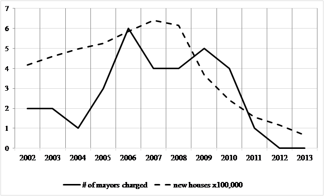
Table 1 reports descriptive statistics of the variables. Figure 1 shows the number of indicted mayors and the number of new houses built in Spain. The trends are somehow correlated, with corruption cases and new houses skyrocketing until 2006-2007, and plummeting afterwards (the huge Spanish property bubble burst in 2008). As we said before, there is some connection between municipal corruption and the colossal urban development occurred in Spain, which brought enormous financial resources to the Spanish municipalities (Benito et al., 2010). In fact, there are claims that urban development should return to the central government in Spain, to prevent local lobbies’ influence on that policy. This feature deserves future research, as we will comment later, in order to investigate whether Goel & Nelson (2011) findings described in the previous paragraph apply to Spain.
Table 1. Descriptive Statistics
| Variable | Description. Source | Obs | Mean | Std. Dev. | Min | Max | |
|---|---|---|---|---|---|---|---|
dependent variable | r_totalexppc | Real total expenditure per capita. Spanish Ministry of Finance. | 1,629 | 798.49 | 220.98 | 370.55 | 2,083.19 |
| r_capitalpc | Real capital expenditure per capita. Spanish Ministry of Finance. | 1,629 | 147.66 | 106.21 | .29 | 954.43 | |
| r_wspc | Real wages and salaries expenditure per capita. Spanish Ministry of Finance. | 1,629 | 281.22 | 75.5412 | 145.00 | 731.05 | |
| r_borrowpc | Real borrowing expenditure per capita. Spanish Ministry of Finance. | 1,630 | 26.08 | 105.39 | -203.56 | 1,307.95 | |
| r_policepc | Real police expenditure per capita. Spanish Ministry of Finance. | 1,553 | 68.31 | 31.57 | 3.03 | 318.41 | |
| r_waterpc | Real water supply/sanitation expenditure per capita. Spanish Ministry of Finance. | 1,148 | 28.11 | 35.87 | 1.03 | 311.57 | |
| r_trashpc | Real trash collection expenditure per capita Spanish Ministry of Finance. | 1,512 | 73.58 | 39.19 | 1.02 | 322.94 | |
| r_educpc | Real education expenditure per capita. Spanish Ministry of Finance. | 1,592 | 40.54 | 31.85 | .25 | 254.51 | |
| r_welfarepc | Real welfare expenditure per capita. Spanish Ministry of Finance. | 1,606 | 91.74 | 41.72 | 3.53 | 362.45 | |
| r_healthpc | Real health expenditure per capita. Spanish Ministry of Finance. | 1,101 | 6.10 | 8.61 | 1.00 | 97.36 | |
independent variables | court1 | Dummy =1 in the year the mayor is taken to court. Value 0 otherwise. Taken from news on press. | 1,632 | .01 | .13 | 0 | 1 |
| court2 | Dummy=1 in the years the corrupt mayor is in power until is taken to court. Value 0 otherwise. Taken from news on press. | 1,632 | .076 | .26 | 0 | 1 | |
| court3 | Dummy=1 in the years the corrupt mayor was in power. Value 0 otherwise. Taken from news on press. | 1,632 | .140 | .34 | 0 | 1 | |
control variables | majority | Majority of a party in municipal council=1; 0 otherwise. Spanish Interior Ministry. | 1,632 | .581 | .49 | 0 | 1 |
| r_grantpc | Real total grants received by the municipality from regional or central governments, per capita Spanish Ministry of Finance. | 1,632 | 279.98 | 96.01 | 0 | 724.46 | |
| MCideology | Municipal Council political sign (0 left; 1 right). Spanish Interior Ministry. | 1,628 | .53 | .49 | 0 | 1 | |
| age_18_64 | Percentage of citizens aged between 18-64 over total. Spanish Statistical Office. | 1,632 | 64.77 | 2.76 | 55.06 | 74.07 | |
| lnpopul | Natural logarithm of municipal population. Spanish Statistical Office. | 1,632 | 11.58 | .74 | 10.43 | 15.00 | |
| munelectionyear | Dummy= 1 election year; 0 otherwise. Spanish Interior Ministry. | 1,632 | .25 | .43 | 0 | 1 | |
| munpreelection | Dummy= 1 pre-election year; 0 otherwise. Spanish Interior Ministry. | 1,632 | .25 | .43 | 0 | 1 | |
| munpostelection | Dummy= 1 post-election year; 0 otherwise. Spanish Interior Ministry. | 1,632 | .25 | .43 | 0 | 1 | |
| income | Municipal disposable personal income, ranges 1-10. Lawrence R. Klein Economic Institute (Madrid). | 1,632 | 6.26 | 2.10 | 2 | 10 | |
16 (N-1) dummy variables autcom*, which account for each municipality’s region, are not reported. Financial variables show 2002 real €.
Figure 1. Number of Mayors Charged with Corruption Per Year
Furthermore, Figure 2 shows the map of mayors’ corruption in Spain. The south part of the country and Atlantic’s Canary Islands have suffered many of the cases of corruption. This regional pattern has been controlled in the regressions through the regional dummy variables autcom*.
Figure 2. Map of Mayors’ Corruption in Spain (2002-2013)
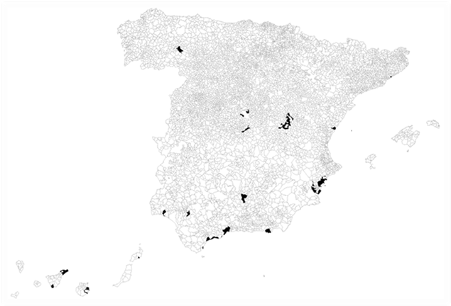
Note: Own elaboration. The municipalities shaded are those reporting one or more cases of corruption during the period analyzed (2002-2013).
Table 2 presents differences between means of all dependent variables, according to the three corruption variables: court1, court2 and court3. In bold we indicate those variables that either confirm or do not significantly reject the sign predicted by the literature. As Table 2 shows, these univariate preliminary tests only reject two assumptions made by the literature, i.e., welfare and health (r_welfarepc and r_healthpc), which the literature states that corruption tends to diminish, but they appear to be higher with corrupt mayors in our data. Regarding education (r_educpc), the literature expects to be diminished by corrupt mayors, but our data shows no statistical difference. These results just show a global picture of our data, and they must be confirmed with the multivariate analysis, i.e., GMM regressions.
Table 2. Difference Between Means of Dependent Variables
| court1 (year in which mayor is charged with corruption) | court1=1 mean (€) | court1=0 mean (€) | t-student difference | expected (literature) | reported (our data) | |
|---|---|---|---|---|---|---|
| (1) | (2) | (3) | (1)-(2) | (1)-(2) | ||
| Corruption means higher expenditure | r_totalexppc | 850.19 | 797.45 | *1.33 | >0 | >0 |
| r_capitalpc | 158.85 | 147.44 | 0.60 | >0 | =0 | |
| r_wspc | 305.21 | 280.74 | **1.81 | >0 | >0 | |
| r_borrowpc | 7.21 | 26.46 | 1.02 | >0 | =0 | |
| r_policepc | 75.45 | 68.16 | *1.29 | >0 | >0 | |
| r_waterpc | 24.22 | 28.17 | -0.48 | >0 | =0 | |
| r_trashpc | 86.94 | 73.30 | **1.92 | >0 | >0 | |
| corruption means lower expenditure | r_educpc | 38.53 | 40.58 | -0.35 | <0 | =0 |
| r_welfarepc | 107.83 | 91.42 | **2.20 | <0 | >0 | |
| r_healthpc | 6.80 | 6.08 | 0.34 | <0 | =0 | |
| court2 (years in power until mayor is charged with corruption) | court2=1 mean (€) | court2=0 mean (€) | t-student difference | expected (literature) | reported (our data) | |
| (1) | (2) | (3) | (1)-(2) | (1)-(2) | ||
| corruption means higher expenditure | r_totalexppc | 869.32 | 792.24 | ***3.85 | >0 | >0 |
| r_capitalpc | 194.95 | 143.49 | ***5.38 | >0 | >0 | |
| r_wspc | 291.67 | 280.30 | **1.65 | >0 | >0 | |
| r_borrowpc | 25.65 | 26.12 | -0.04 | >0 | =0 | |
| r_policepc | 73.43 | 67.86 | **1.91 | >0 | >0 | |
| r_waterpc | 36.83 | 27.40 | ***2.35 | >0 | >0 | |
| r_trashpc | 80.94 | 72.92 | **2.19 | >0 | >0 | |
| corruption means lower expenditure | r_educpc | 44.11 | 40.25 | 1.27 | <0 | =0 |
| r_welfarepc | 107.56 | 90.37 | ***4.49 | <0 | >0 | |
| r_healthpc | 7.84 | 5.95 | **1.91 | <0 | >0 | |
| court3 (all years mayor charged with corruption is in power) | court3=1 mean (€) | court3=0 mean (€) | t-student difference | expected (literature) | reported (our data) | |
| (1) | (2) | (3) | (1)-(2) | (1)-(2) | ||
| corruption means higher expenditure | r_totalexppc | 844.17 | 790.48 | ***3.50 | >0 | >0 |
| r_capitalpc | 165.84 | 144.47 | ***2.89 | >0 | >0 | |
| r_wspc | 297.10 | 278.44 | ***3.56 | >0 | >0 | |
| r_borrowpc | 23.73 | 26.49 | 0.37 | >0 | =0 | |
| r_policepc | 69.46 | 68.12 | 0.59 | >0 | =0 | |
| r_waterpc | 34.37 | 27.25 | **2.19 | >0 | >0 | |
| r_trashpc | 80.17 | 72.43 | ***2.20 | >0 | >0 | |
| corruption means lower expenditure | r_educpc | 38.08 | 40.95 | 1.26 | <0 | =0 |
| r_welfarepc | 99.54 | 90.38 | ***3.14 | <0 | >0 | |
| r_healthpc | 7.28 | 5.91 | **1.79 | <0 | >0 | |
5.2. Specification of the model
In line with previous literature and the structure of our panel data, we use the following GMM equation (Liu & Mikesell, 2014):
\[\begin{equation} \label{eq1} \small y_{it}= \gamma + \alpha y_{it-1} + \sum \beta_{j}x_{jit}+c_{i}+\varepsilon_{it} \ \ \ \ (1) \end{equation}\]
Where yit represents each of the spending categories discussed previously (see first half of Table 1). Following Dezhbakhsh et al. (2003), budget figures usually follow an incremental approach. To control for this budgetary inertia, we include the lagged dependent variable as regressor (\(\alpha y_{it-1}\)). \(\gamma\) is the intercept, xjit is the vector of explanatory variables and \(\beta_{j}\) is a vector of parameters to be estimated (see second half of Table 1). To control for fixed municipal effects (unobserved heterogeneity), we introduce ci. The error term is \(\varepsilon_{it}\). Subscripts i and t represent municipality (1 to 145) and time (2002 to 2013), respectively.
Blundell & Bond (1998) state that with persistent series, i.e., when current value of variables is determined mostly by their previous value, differenced GMM estimator reports important sample biases and imprecision. We must bear in mind that budget figures usually follow an incremental approach, as we said before, which means a budgetary inertia (Dezhbakhsh et al., 2003). Thus, we assume that our data are persistent (stationary). To control for this problem, we tested the persistence of our variables using the Levin et al. (2002) method and confirmed its results with Harris & Tzavalis (1999) and Breitung (2000) in case the first method did not confirm stationary (Levin method requires quite restrictive assumptions). We find overwhelming evidence against the null hypothesis of a unit root and therefore we conclude that our variables are stationary, which implies that the system GMM estimation will provide more precise analysis than the difference GMM for our data.
5.3. Results and robustness checks
Tables 3, 4 and 5 show system GMM regressions with independent variables court1, court2 and court3, respectively.
Table 3. Impact of Mayor’s Corruption (court1) on Municipal Spending per Capita, 2002–2013, System GMM
| dependent variable | r_totalexppc | r_capitalpc | r_wspc | r_borrowpc | r_policepc | r_waterpc | r_trashpc | r_educpc | r_welfarepc | r_healthpc |
|---|---|---|---|---|---|---|---|---|---|---|
| expected sign of court1 | (+) | (+) | (+) | (+) | (+) | (+) | (+) | (-) | (-) | (-) |
| court1 | **308.76 2.36 | **101.75 2.19 | **37.14 2.44 | -42.73 -0.88 | 17.58 1.22 | -2.90 -0.13 | ***76.49 2.79 | **33.76 2.49 | 15.80 0.87 | -2.37 -0.32 |
| dependent variablet-1 | ***.51 12.16 | ***.31 4.93 | ***.83 29.61 | ***-.20 -6.82 | ***.67 16.07 | ***.38 2.77 | ***.49 8.55 | ***.52 7.72 | ***.64 21.51 | ***.57 4.45 |
| majority | 9.11 1.01 | **12.31 2.35 | 2.55 1.53 | 2.71 0.27 | 1.68 1.29 | .09 0.05 | .52 0.27 | .01 0.01 | 2.55 1.39 | -.34 -1.50 |
| r_grantpc | ***.50 6.96 | ***.41 8.41 | ***.03 2.70 | **.10 2.11 | -.01 -1.21 | .01 0.98 | ***-.04 -3.93 | ***.04 6.33 | ***.05 4.36 | .00 0.47 |
| MCideology | -6.57 -0.57 | -8.79 -1.44 | ***-5.39 -2.71 | 12.06 1.56 | -2.04 -1.48 | -.02 -0.01 | -1.65 -0.72 | 1.57 1.14 | ***-6.65 -3.06 | -.45 -1.10 |
| age_18_64 | ***6.15 2.79 | .42 0.38 | .55 1.03 | 1.06 0.62 | .21 0.84 | .26 0.39 | ***1.42 3.27 | -.20 -0.88 | .34 0.92 | .02 0.35 |
| lnpopul | ***-30.64 -3.94 | ***-24.36 -4.82 | ***-4.28 -2.89 | -4.88 -0.77 | 1.53 1.23 | **-4.87 -2.07 | -1.61 -1.03 | ***-3.89 -3.69 | ***-4.21 -2.85 | .03 0.16 |
| munelectionyear | -7.6043 -0.87 | 3.07 0.46 | ***-5.06 -2.83 | -2.40 -0.36 | ***-3.43 -3.18 | **-3.52 -2.12 | ***-4.29 -3.06 | ***3.62 3.36 | -.85 -0.60 | .18 0.59 |
| munpreelection | ***-61.49 -6.58 | ***-25.77 -4.23 | ***-12.70 -6.19 | -5.67 -0.88 | ***-7.51 -5.67 | -2.55 -0.99 | ***-11.11 -5.07 | .20 0.19 | ***-13.31 -7.89 | -.44 -0.97 |
| munpostelection | ***-27.50 -2.94 | ***-19.93 -3.37 | ***-10.62 -4.80 | ***36.46 5.83 | ***-3.96 -3.79 | *-3.88 -1.86 | -2.65 -1.55 | 1.31 1.46 | ***-6.08 -5.25 | -.35 -1.08 |
| income | ***39.66 9.03 | ***14.95 7.41 | ***6.48 7.69 | -3.41 -0.84 | ***3.03 6.40 | .94 1.28 | ***5.99 6.33 | *.86 1.87 | ***5.05 6.32 | **.46 2.52 |
| AR test | z = -0.04 Pr = 0.96 | z = -1.62 Pr = 0.10 | z = 1.60 Pr = 0.10 | z = 2.00 Pr = 0.04 | z = -0.26 Pr = 0.79 | z = 1.39 Pr = 0.16 | z = -0.90 Pr = 0.37 | z = 0.42 Pr = 0.67 | z = -0.69 Pr = 0.48 | z = 1.46 Pr = 0.14 |
| Hansen test | chi2=116.3 Prob = 0.14 | chi2=119.9 Prob = 0.70 | chi2= 130.4 Prob = 0.35 | chi2=111.1 Prob = 0.12 | chi2=113.1 Prob = 0.25 | chi2=96.88 Prob = 0.48 | chi2=110.39 Prob = 0.31 | chi2=110.93 Prob = 0.30 | chi2=116.19 Prob = 0.19 | chi2=87.37 Prob = 0.91 |
Panel-data | LLC= .000 | LLC= .000 | LLC= .000 | LLC= 1.000 HT= .000 B= .000 | LLC= 0.087 HT= .000 B= .000 | LLC= 0.006 | LLC= 0.921 HT= .000 B= .000 | LLC= .000 | LLC= 0.490 HT= .002 B= .000 | LLC= .000 |
Variable court1 is a dummy with value 1 in the year the mayor is indicted and value 0 in the remaining years. All models include:
A constant (not shown).
16 (N-1) dummy variables autcom*, which account for each municipality’s region (not shown).
Financial variables show 2002 real €. Below each coefficient, z value is reported. Significance: *10%, **5%, ***1%.
Panel-data unit-root tests p-values (stationary): Levin, Lin and Chu (2002): LLC; Harris and Tzavalis (1999): HT; Breitung (2000): B.
Table 4. Impact of Mayor’s Corruption (court2) on Municipal Spending per Capita, 2002–2013, System GMM
| dependent variable | r_totalexppc | r_capitalpc | r_wspc | r_borrowpc | r_policepc | r_waterpc | r_trashpc | r_educpc | r_welfarepc | r_healthpc |
|---|---|---|---|---|---|---|---|---|---|---|
| expected sign of court2 | (+) | (+) | (+) | (+) | (+) | (+) | (+) | (-) | (-) | (-) |
| court2 | ***80.85 3.79 | ***100.13 4.25 | **14.16 2.47 | -9.49 -0.50 | ***10.77 3.25 | 6.81 0.57 | **14.73 2.25 | 6.59 1.32 | **12.92 2.22 | .65 0.64 |
| dependent variablet-1 | ***.52 12.75 | ***.28 4.33 | ***.83 29.88 | ***-.19 -6.90 | ***.66 14.85 | ***.38 2.94 | ***.49 8.32 | ***.53 7.19 | ***.64 20.37 | ***.60 4.89 |
| majority | 11.22 1.28 | *10.11 1.78 | 2.57 1.47 | 2.04 0.23 | .84 0.69 | .16 0.10 | .04 0.02 | -.17 -0.13 | **3.52 2.01 | -.30 -0.77 |
| r_grantpc | ***.50 7.23 | ***.47 8.95 | ***.03 2.89 | **.11 2.49 | -.01 -1.09 | .00 0.65 | ***-.03 -3.61 | ***.05 6.44 | ***.06 4.75 | .00 0.01 |
| MCideology | -9.80 -0.88 | -6.23 -0.92 | **-5.24 -2.53 | 10.98 1.45 | *-1.95 -1.67 | -.51 -0.27 | -2.65 -1.19 | 1.37 1.00 | ***-6.62 -3.28 | -.60 -1.20 |
| age_18_64 | ***7.53 3.62 | 1.49 1.33 | .78 1.39 | 1.13 0.75 | .40 1.42 | .44 0.55 | ***1.60 3.42 | -.16 -0.66 | .46 1.31 | -.01 -0.12 |
| lnpopul | ***-27.64 -3.45 | ***-22.67 -4.39 | **-3.80 -2.51 | -6.12 -0.91 | 1.55 1.14 | **-4.11 -2.14 | -1.74 -0.99 | ***-3.14 -2.62 | ***-4.12 -3.06 | -.00 -0.01 |
| munelectionyear | -8.59 -0.97 | 7.66 1.10 | ***-5.23 -2.81 | -6.32 -1.02 | ***-3.44 -3.24 | **-3.57 -2.03 | ***-4.10 -2.83 | ***3.87 3.29 | -.96 -0.74 | .23 0.53 |
| munpreelection | ***-56.03 -7.23 | ***-23.67 -4.18 | ***-12.09 -6.05 | -8.59 -1.53 | ***-7.83 -6.12 | -2.33 -0.86 | ***-10.81 -5.38 | .75 0.82 | ***-13.10 -7.77 | -.45 -0.77 |
| munpostelection | ***-32.92 -3.65 | ***-18.76 -3.11 | ***-11.32 -4.75 | ***34.50 5.52 | ***-4.38 -4.40 | *-4.07 -1.73 | *-2.87 -1.71 | 1.46 1.55 | ***-6.33 -5.45 | -.32 -0.73 |
| income | ***39.11 10.29 | ***11.88 5.14 | ***6.05 7.99 | -3.84 -0.96 | ***3.14 6.40 | *1.35 1.73 | ***6.07 6.50 | .44 0.97 | ***4.53 5.49 | .36 1.44 |
| AR test | z = -0.22 Pr = 0.82 | z = -1.79 Pr = 0.07 | z = 1.56 Pr = 0.12 | z = 1.53 Pr = 0.13 | z = -0.21 Pr = 0.84 | z = 1.32 Pr = 0.19 | z = -0.59 Pr = 0.55 | z = 0.48 Pr = 0.63 | z = -0.79 Pr = 0.42 | z = 1.48 Pr = 0.14 |
| Hansen test | chi2=123.06 Prob = 0.09 | chi2=121.35 Prob = 0.67 | chi2=131.23 Prob = 0.38 | chi2=113.71 Prob = 0.09 | chi2=118.57 Prob = 0.19 | chi2=92.43 Prob = 0.74 | chi2=113.87 Prob = 0.28 | chi2=114.44 Prob = 0.27 | chi2=114.28 Prob = 0.27 | chi2=88.89 Prob = 0.83 |
Variable court2 is a dummy with value 1 all years the mayor has been in office until the year in which is indicted, and takes value 0 the remaining years. All models include:
A constant (not shown).
16 (N-1) dummy variables autcom*, which account for each municipality’s region (not shown).
Financial variables show 2002 real €. Below each coefficient, z value is reported. Significance: *10%, **5%, ***1%.
Table 5. Impact of Mayor’s Corruption (court3) on Municipal Spending per Capita, 2002–2013, System GMM
| dependent variable | r_totalexppc | r_capitalpc | r_wspc | r_borrowpc | r_policepc | r_waterpc | r_trashpc | r_educpc | r_welfarepc | r_healthpc |
|---|---|---|---|---|---|---|---|---|---|---|
| expected sign of court3 | (+) | (+) | (+) | (+) | (+) | (+) | (+) | (-) | (-) | (-) |
| court3 | ***77.91 3.46 | 15.99 0.86 | **10.17 2.09 | -25.44 -1.07 | 5.50 1.39 | 7.63 0.65 | 9.93 1.51 | 3.51 0.78 | *5.97 1.86 | -.99 -0.82 |
| dependent variablet-1 | ***.51 12.53 | ***.28 4.21 | ***.83 27.95 | ***-.21 -6.07 | ***.67 16.43 | ***.39 2.78 | ***.48 8.14 | ***.53 6.78 | ***.65 21.26 | ***.59 4.85 |
| majority | 7.47 0.82 | 10.11 1.61 | 1.92 1.12 | 8.11 0.80 | 1.13 0.94 | .33 0.17 | -.25 -0.12 | -.64 -0.45 | **3.76 2.23 | -.22 -0.48 |
| r_grantpc | ***.49 6.99 | ***.48 8.45 | ***.03 2.93 | **.10 2.15 | *-.01 -1.80 | .00 0.28 | ***-.03 -3.72 | ***.04 5.68 | ***.05 4.68 | .00 0.11 |
| MCideology | -13.10 -1.10 | -7.35 -1.01 | **-5.42 -2.50 | 10.30 1.44 | *-2.17 -1.84 | -.79 -0.40 | -3.17 -1.37 | 1.10 0.80 | ***-7.63 -3.91 | -.59 -1.27 |
| age_18_64 | ***6.95 3.39 | .53 0.38 | .64 1.17 | .57 0.35 | .36 1.42 | .50 0.56 | ***1.59 3.52 | -.25 -1.06 | .44 1.33 | -.01 -0.28 |
| lnpopul | ***-26.81 -3.10 | ***-26.07 -4.43 | ***-4.14 -2.64 | -5.13 -0.76 | 1.73 1.29 | *-3.99 -1.82 | -2.05 -1.10 | ***-3.40 -2.83 | **-3.40 -2.44 | -.02 -0.05 |
| munelectionyear | -8.94 -1.13 | 3.22 0.44 | ***-5.39 -2.75 | -3.20 -0.49 | ***-3.62 -3.72 | *-3.91 -1.95 | ***-4.87 -3.37 | ***3.67 2.76 | -1.41 -1.06 | .20 0.47 |
| munpreelection | ***-56.15 -6.76 | ***-24.94 -3.83 | ***-12.19 -5.71 | -3.96 -0.65 | ***-7.14 -5.97 | -2.68 -0.90 | ***-11.45 -6.04 | .93 1.00 | ***-13.09 -8.11 | -.54 -0.89 |
| munpostelection | ***-29.77 -3.33 | ***-17.64 -2.73 | ***-10.97 -4.66 | ***32.32 5.68 | ***-4.44 -4.95 | *-4.14 -1.68 | **-3.41 -2.00 | 1.42 1.43 | ***-6.32 -5.60 | -.31 -0.88 |
| income | ***36.85 9.06 | ***16.98 5.83 | ***5.85 8.00 | -.14 -0.04 | ***3.07 6.80 | *1.44 1.60 | ***6.22 6.96 | .42 0.82 | ***4.16 5.65 | *.46 1.79 |
| AR test | z = -0.24 Pr = 0.81 | z = -1.23 Pr = 0.22 | z = 1.56 Pr = 0.12 | z = 1.59 Pr = 0.11 | z = -0.19 Pr = 0.85 | z = 1.35 Pr = 0.18 | z = -0.51 Pr = 0.61 | z = 0.52 Pr = 0.60 | z = -0.58 Pr = 0.56 | z = 1.44 Pr = 0.15 |
| Hansen test | chi2=119.84 Prob = 0.08 | chi2=115.87 Prob = 0.11 | chi2=131.78 Prob = 0.24 | chi2=106.12 Prob = 0.13 | chi2=107.36 Prob = 0.27 | chi2=97.33 Prob = 0.53 | chi2=112.22 Prob = 0.17 | chi2=112.71 Prob = 0.16 | chi2=108.48 Prob = 0.24 | chi2=91.37 Prob = 0.67 |
Variable court3 takes value 1 for all years of mandate of the corrupt mayor, even after being charged with corruption, and value 0 in the remaining years.
All models include:
A constant (not shown).
16 (N-1) dummy variables autcom*, which account for each municipality’s region (not shown).
Financial variables show 2002 real €. Below each coefficient, z value is reported. Significance: *10%, **5%, ***1%.
Table 3 presents unit root checks to evaluate stationarity of dependent variable time series, which for the sake of simplicity are not repeated on tables 4 and 5. To provide robustness checks, we report two additional analyses.
First, we run again system GMM regressions with the same independent variables but we replace each per capita dependent variable with the percentage of every spending item over the total municipal spending, i.e., whether mayors are prioritizing one particular spending item because it is easier to get payoffs, out of the total budget (see Table 6).
Second, we keep all system GMM variables but we run ordinary least squares regressions (OLS) with cluster-robust errors, instead of system GMM (Liu & Mikesell, 2014). We suspect that OLS is biased because of the municipality’s fixed effects (unobserved heterogeneity) and the endogeneity of corruption (Liu & Mikesell, 2014). Anyway, coefficients that remain significant in under OLS reinforce their robustness (see Table 7).
For the sake of simplicity, Tables 6 and 7 only show the main independent variables, i.e., court1, court2 and court3. Full regressions are available upon request to the authors.
Table 6. Impact of Mayor’s Corruption on Municipal Spending Percentage Over Total, 2002–2013, System GMM
| dependent variable | capitalperc | wsperc | borrowperc | policeperc | waterperc | trashperc | educperc | welfareperc | healthperc |
|---|---|---|---|---|---|---|---|---|---|
| expected sign of court# | (+) | (+) | (+) | (+) | (+) | (+) | (-) | (-) | (-) |
| court1 | **.08 1.93 | -.02 -0.59 | -.07 -1.06 | .00 0.32 | .01 0.33 | **.06 2.31 | *.02 1.75 | .00 0.22 | .00 .04 |
| AR test | z = -1.46 Pr = 0.14 | z = -0.67 Pr = 0.51 | z = 2.41 Pr = 0.02 | z = -0.01 Pr = 0.99 | z = 1.08 Pr = 0.28 | z = -0.40 Pr = 0.69 | z = -0.22 Pr = 0.82 | z = -0.66 Pr = 0.51 | z = -1.40 Pr = 0.16 |
| Hansen test | chi2=125.48 Prob = 0.57 | chi2=123.57 Prob = 0.52 | chi2=118.98 Prob = 0.05 | chi2=102.65 Prob = 0.52 | chi2=66.46 Prob = 0.56 | chi2=101.26 Prob = 0.56 | chi2=111.40 Prob = 0.29 | chi2=97.70 Prob = 0.66 | chi2=98.11 Prob = 0.72 |
| court2 | ***.07 3.61 | -.01 -1.40 | -.03 -1.16 | **0.01 1.94 | .01 0.57 | .01 1.15 | .00 0.43 | .01 1.03 | .00 .13 |
| AR test | z = -1.55 Pr = 0.12 | z = -0.60 Pr = 0.55 | z = 2.06 Pr = 0.04 | z = -0.01 Pr = 0.98 | z = 1.09 Pr = 0.28 | z = 0.03 Pr = 0.97 | z = -0.05 Pr = 0.95 | z = -0.69 Pr = 0.49 | z = 1.75 Pr = 0.08 |
| Hansen test | chi2=126.09 Prob = 0.56 | chi2=123.32 Prob = 0.58 | chi2=118.36 Prob = 0.05 | chi2=100.39 Prob = 0.64 | chi2=66.41 Prob = 0.72 | chi2=110.25 Prob = 0.37 | chi2=113.83 Prob = 0.28 | chi2=95.89 Prob = 0.75 | chi2=98.74 Prob = 0.60 |
| court3 | 0.00 0.38 | -.00 -0.21 | *-.05 -1.72 | .00 0.85 | .01 0.92 | .01 0.92 | -.00 -0.07 | .00 0.40 | -.00 -.87 |
| AR test | z = -1.62 Pr = 0.11 | z = -0.69 Pr = 0.49 | z = 2.06 Pr = 0.04 | z = -0.02 Pr = 0.95 | z = 1.10 Pr = 0.27 | z = 0.08 Pr = 0.94 | z = -0.03 Pr = 0.97 | z = -0.63 Pr = 0.53 | z = 1.75 Pr = 0.08 |
| Hansen test | chi2=127.67 Prob = 0.39 | chi2=125.49 Prob = 0.37 | chi2=114.54 Prob = 0.05 | chi2=103.09 Prob = 0.37 | chi2=64.70 Prob = 0.69 | chi2=103.82 Prob = 0.35 | chi2=109.37 Prob = 0.22 | chi2=93.96 Prob = 0.62 | chi2=93.81 Prob = 0.60 |
Variable court1 is a dummy with value 1 in the year in which the mayor is taken to court and value 0 in the remaining years.
Variable court2 is a dummy that takes value 1 during all years the mayor has been in office until the year in which is taken to court, and takes value 0 the remaining years.
Variable court3 takes value 1 for all years of mandate of the corrupt mayor, even after being charged with corruption, and value 0 in the remaining years.
All models include:
A constant (not shown).
16 (N-1) dummy variables autcom*, which account for each municipality’s region (not shown).
Financial variables show 2002 real €. Below each coefficient, z value is reported. Significance: *10%, **5%, ***1%.
Table 7. Impact of Mayor’s Corruption on Spending per Capita, 2002–2013, OLS with cluster-robust errors
| dependent variable | r_totalexppc | r_capitalpc | r_wspc | r_borrowpc | r_policepc | r_waterpc | r_trashpc | r_educpc | r_welfarepc | r_healthpc |
|---|---|---|---|---|---|---|---|---|---|---|
| expected sign of court# | (+) | (+) | (+) | (+) | (+) | (+) | (+) | (-) | (-) | (-) |
| court1 | -7.48 -0.36 | -7.08 -0.56 | 7.97 1.18 | -18.40 -1.45 | -1.71 -0.55 | -5.04 -1.04 | 5.63 1.06 | .52 0.19 | 6.70 1.18 | -3.32 -1.15 |
| R2 | 0.79 | 0.58 | 0.92 | 0.07 | 0.80 | 0.59 | 0.66 | 0.80 | 0.78 | 0.70 |
| court2 | ***31.83 2.82 | ***24.03 2.90 | ***8.88 3.13 | -6.25 -0.58 | **3.50 2.17 | .18 0.06 | 3.90 1.16 | 1.58 0.76 | ***7.74 3.05 | -.38 -0.37 |
| R2 | 0.79 | 0.58 | 0.92 | 0.07 | 0.80 | 0.59 | 0.66 | 0.80 | 0.78 | 0.70 |
| court3 | 8.79 1.03 | 7.37 1.25 | 3.09 1.52 | -10.72 -1.22 | -.58 -0.46 | .06 0.03 | .86 0.38 | .17 0.12 | 2.05 1.14 | -.99 -1.33 |
| R2 | 0.79 | 0.58 | 0.92 | 0.07 | 0.80 | 0.59 | 0.66 | 0.80 | 0.78 | 0.70 |
court1 is a dummy with value 1 in the year in which the mayor is taken to court and value 0 in the remaining years.
court2 is a dummy that takes value 1 during all years the mayor has been in office until the year in which is taken to court, and takes value 0 the remaining years.
court3 takes value 1 for all years of mandate of the corrupt mayor, even after being charged with corruption, and value 0 in the remaining years.
All models include:
A constant (not shown).
16 (N-1) dummy variables autcom*, which account for each municipality’s region (not shown).
Financial variables show 2002 real €. Below each coefficient, t value. Significance: *10%, **5%, ***1%.
The stationarity of the dependent variables is again confirmed by the value of the lagged dependent variable, which ranges between 0 and 1 in all regressions (see dependent variablet-1 on Tables 3, 4 and 5). Besides, it is 1% significant in all the regressions, which proves the budgetary inertia posited by Dezhbakhsh et al. (2003). Moreover, population (lnpopul) presents, in all significant cases, a negative sign, which indicates economies of scale in municipal expenditures in Spain. Finally, the Wagner’s law is confirmed through the positive, significant coefficient of the variable income, which proves the economic rationality of our data.
6. Discussion
6.1. Total expenditure
Our coefficients show that corrupt mayors increase total expenditure in all definitions of corruption: court1, court2 and court3, i.e., during all years they are in power, even after being indicted with corruption (variable r_totalexppc, Tables 3, 4 and 5). The latter does not agree with the results of Artés et al. (2015), who, for a sample of Spanish municipalities, show that, after corruption is revealed, investment expenditures decrease significantly.
We now consider both differences between means (Table 2) and regressions (Tables 3, 4 and 5) to report € impact of corruption. Thus, the year the mayor is indicted (court1), total expenditure per capita is between €52.73 and €308.76 higher. If we consider court2, total expenditure per capita is between €77.08 and €80.85 higher. If we consider court3, total average expenditure per capita is between €53.69 and €77.91 greater.
We confirm that the budget is a sum of allocated spending plus bribes (Tanzi, 1998), and that corruption involves the whole budget (Rose-Ackerman, 1999), which is maximized for mayors’ private gain (Liu & Mikesell, 2014). However, we find that corrupt mayors spend 10.13 percent more, which is lower than the 18 percent found by Rose-Ackerman (1999).
Regarding the robustness of the results, impact of court2 on total expenditure is significant under system GMM and OLS (variable r_totalexppc, Table 7). This is a strong indicator, considering how restrictive OLS is in terms of significance of coefficients.
6.2. Capital
Our data show that corrupt mayors spend more on capital projects, both on a per capita basis (r_capitalpc, Tables 3, 4 and 5), and as percentage over total spending (capitalperc, Table 6). This result confirms Tanzi & Davoodi (1997) and Liu & Mikesell (2014) findings, which show that corruption increases public investment projects because these projects allow manipulations to get bribes.
However, both on a per capita basis and as percentage over total, only court1 and court2 are significant (only court2 in OLS models). This means that corrupt mayors refrain from manipulating capital expenditures after being indicted, since they know their capital budget management will be scrutinized. In fact, Artés et al. (2015) find that, in Spain, capital expenditures decrease after revealing corruption scandals in the municipality.
Corruption requires secrecy, which shifts appropriations away from health and education, into potentially useless projects, such as infrastructure (Shleifer & Vishny, 1993). These projects are sometimes “white elephant” projects with little real value (Mauro, 1998). Unfortunately, these “white elephant” projects have been common in Spanish municipalities.
6.3. Police and wages and salaries
Our results indicate overspending on police before the mayor is indicted (court2), both per capita (r_policepc, Tables 3, 4, 5) and percentage over total (policeperc, Table 6). In per capita terms, this means between €5.57 and €10.77 (Tables 2 and 4, respectively). We prove that mayors use the machinery of government to provide jobs for supporters. We must bear in mind that police service is an area with many patronage jobs (Rose-Ackerman, 1999).
Regarding total wages and salaries per capita, we find an impact of mayor’s corruption (variable r_wspc, Tables 3, 4 and 5) in all the corruption variables (court1, court2, court3). The same result is found in the univariate analysis of difference between means (Table 2) and on the OLS model for court2 (Table 7). However, results do not hold on percentages over total (wsperc, Table 6). Therefore, our results in this regard are not conclusive.
6.4. Borrowing
Corrupt public officials may have stronger incentives to create fiscal illusions through debt, as a way to make citizens underestimate their real fiscal burdens, both present and future (Liu & Mikesell, 2014). Though the literature predicts that state and local governments’ debt appears to be higher as corruption increases, we find no significant impact of mayors’ corruption on the municipal debt growth (variable r_borrowpc, Tables 3, 4 and 5). The greater expenditure per capita is funded partly with central and regional government transfers received by corrupt mayors’ municipalities (variable r_grantpc, Table 8), since tax revenues per capita are not significantly greater in corrupt municipalities (see Table 9).
Table 8. Difference Between Means: r_grantpc
| court1 | court1=1 mean (€) | court1=0 mean (€) | t-student difference |
| r_grantpc | 298.94 | 279.60 | 1.13 |
| court2 | court2=1 mean (€) | court2=0 mean (€) | t-student difference |
| r_grantpc | 297.11 | 278.47 | **2.14 |
| court3 | court3=1 mean (€) | court3=0 mean (€) | t-student difference |
| r_grantpc | 296.29 | 277.12 | ***2.87 |
Table 9. Difference Between Means: municipal taxes, fees per capita
| court1 | court1=1 mean (€) | court1=0 mean (€) | t-student difference |
| municipal taxes and fees per capita | 496.78 | 485.33 | 0.39 |
| court2 | court2=1 mean (€) | court2=0 mean (€) | t-student difference |
| municipal taxes and fees per capita | 495.59 | 484.67 | 0.73 |
| court3 | court3=1 mean (€) | court3=0 mean (€) | t-student difference |
| municipal taxes and fees per capita | 489.38 | 484.89 | 0.39 |
6.5. Sewer, water and trash collection
Our data show only an impact of corruption on trash collection expenditures per capita (r_trashpc, Tables 3, 4 and 5) before the mayor is charged (variables court1 and court2). In the percentage model (trashperc, Table 6), only court1 is significant, which means that in the year the mayor is charged, this kind of expenditure is manipulated with the aim of getting payoffs. In this sense, the mayors involved in corruption cases by obtaining, on many occasions, a personal benefit from the private companies that manage this municipal service, may be neglecting the efficient management of this service, which increases its cost (Liu & Mikesell, 2014). We confirm previous works such as Hessami (2014), who finds evidence for corruption connected to expenditures on waste management.
Regarding water supply and sanitation, our data are in line with Rose-Ackerman (1999), who does not connect sewers, and water expenditures with corruption (r_waterpc on Tables 3, 4, 5 and 7; waterperc on Table 6).
6.6. Education
Education spending, according to the literature, is one of the activities with low rent extraction potential (Mauro, 1998; Fisman & Gatti, 2002). Thus, some authors even predict that corrupt governments will reduce the portion of education in government expenditure (Shleifer and Vishny, 1993; Delavallade, 2006; De la Croix & Delavallade, 2009). Our data do not show a negative impact on education, they only indicate that the year the mayor is charged, it appears to be a small increase in education expenses (variable r_educpc, Table 3 and variable educperc, Table 6).
&Our coefficients appear to show a positive impact of mayors’ corruption on social protection. Indeed, court2 and court3 present significant impact on per capita basis (variable r_welfarepc, Tables 4 and 5), while both are not significant on the system GMM percentage model (variable welfareperc, Table 6). These results weakly confirm Mauro (1998), who posits positive impact of corruption on welfare payments. It appears mayors are increasing social protection expenses to counteract the effect of their corruption charges among the citizens.
6.7. Health
The literature presents evidence that corruption means less health expenditure (Shleifer & Vishny, 1993; Mauro, 1998; Delavallade, 2006; De la Croix & Delavallade, 2009). Our data do not confirm this assumption, but they just indicate that corrupt mayors are not manipulating health spending (no significant impact of court1, court2 and court3 on r_healthpc on Tables 3, 4, 5 and on healthperc on Table 6).
7. Conclusions and policy implications
We show that total expenditure per capita is between €52.73 and €308.76 higher in municipalities ruled by mayors charged with corruption. We also find an impact of mayors’ corruption on these expenditure items per capita: capital, police and trash collection. The three latter expenditures are reduced after corruption charges are reported by the press. However, total expenditure per capita appears to be higher even after that moment. This indicates that indicted mayors keep on manipulating total expenditure per capita, but they shift appropriations from highly scrutinized items to others.
We agree with Larmour & Wolanin (2013) in that governments have a public duty to reduce corruption. Furthermore, as major purchasers of services in the community, they have the power to influence the behavior of those they deal with, leading by example. This would be achieved if new legislation prevented mayors who leave politics from joining companies that previously implemented capital expenditures, which our data show as connected to corruption.
Another policy implication is in line with Mauro (1998), i.e., governments should improve the composition of their expenditure by increasing the share of those spending categories that are less susceptible to corruption.
Mayors have a paramount role in curbing corruption. The first front in a strategy to fight against corruption should be “honest and visible commitment by the leadership to the fight against corruption, for which the leadership must show zero tolerance” (Tanzi, 1998). This point makes clear that mayors’ corruption is especially harmful for the governance and trustworthiness of municipalities and local economies in general.
Regarding policy implications within the secondary corruption posited by the political elasticity theory, we propose several measures to curb municipal corruption in Spain. First, the Government Accounting Office should focus on these municipal expenditures when auditing municipal financial statements: capital expenditures, police and trash collection. Second, new legislation should scrutinize “white elephant” capital projects by requiring authorization, independent cost-benefit analysis and monitoring from the central government if the investment exceeds certain percentage of the total municipal budget. Third, corrupt mayors’ higher total expenditure per capita is funded partly through grants received from regional or central governments. These governments should better monitor whether the money transferred to municipalities is properly spent.
We must acknowledge some limitations of this study. One limitation may stem from the measurement of corruption. We use the information published by online press about mayors have been taken to court, charged with corruption, to build our corruption variables. However, this information is not normally contrasted by supranational organizations. Moreover, the information provided by these media does not make it possible to differentiate by type of corruption. That is to say, we cannot know exactly for what specific facts the mayor has been accused of corruption. Furthermore, the information published by online press does not always allow us to know how many years mayors have been involved in corruption cases.
Given the above limitations, further research is needed to build a new measure of corruption at local level that takes into account all these issues. Moreover, this new indicator should be built for more municipalities and more years, since, in recent years, local corruption cases have increased. Finally, we think that the relationship between corruption and urban development, suggested on Figure 1, deserves some in depth analyses.