IFRS 9 Expected Loss: A Model Proposal for Estimating the Probability of Default for non-rated companies

ABSTRACT

Under the IFRS 9 impairment model, entities must estimate the PD (Probability of Default) for all financial assets (and other elements) not measured at fair value through profit or loss. There are several methodologies for estimating this PD from market or historical information. However, in some cases entities do not possess market or historical information concerning a counterparty. For such cases, we propose a model called Financial Ratios Scoring (FRS), by means of which an entity can obtain a “shadow rating” for a counterparty as a first step in estimating the PD. The model differentiates from other recent models in several aspects, such as the size of the database and the fact that it is focused on non-rated companies, for example. It is based on scoring the counterparty according to its key financial ratios. The score will place the counterparty on a percentile within a previously constructed sector distribution using companies with a credit rating published by rating agencies or financial vendors. We have tested the model reliability by calculating the internal credit rating of several companies (which have an official/quoted credit rating), and by comparing the rating obtained with the official one, and obtained positive results.

Pérdida prevista según la NIIF 9: una propuesta de modelo para la estimaciónde la probabilidad de impago en las empresas sin rating

RESUMEN

Bajo el modelo de provisiones por riesgo de crédito de la NIIF 9, las empresas deben estimar una Probabilidad de Default o quiebra (PD) para todos los activos financieros (y otros elementos) no valorados a valor razonable con cambios en la cuenta de resultados. Existen varias metodologías para estimar dicha PD utilizando información histórica o de mercado. No obstante, en algunos casos las empresas no disponen de información histórica o de mercado acerca de una contraparte. Para estos casos proponemos un modelo denominado Financial Ratios Scoring (FRS), a través del cual la entidad puede obtener un rating interno de la contraparte como primer paso para estimar la PD. El modelo se diferencia de otros modelos recientes en varios aspectos como, por ejemplo, el tamaño de la base de datos o el hecho de que se enfoca en empresas sin rating. Se basa en dar una puntuación a la contraparte en función de sus ratios financieros clave. La puntuación sitúa a la empresa en un percentil dentro de una distribución del sector previamente construida utilizando empresas con rating oficial u ofrecido por vendors. Hemos analizado la fiabilidad del modelo calculando el rating interno para empresas con rating oficial y hemos comparado el rating interno con el oficial, obteniendo resultados positivos.

1 Introduction

Under International Financial Reporting Standards (IFRS) issued by the International Accounting Standards Boards (IASB), accounting rules for financial instruments have recently changed. International Accounting Standard (IAS) 39 (issued in 1998 and in force since 2001) has been replaced by IFRS 9 for reporting periods beginning on or after 1 January 2018 (earlier application was permitted).

IFRS 9 has introduced several changes. For example, the categories for financial assets are different to those of IAS 39 (classification criteria is also different), and changes have been made to hedge accounting rules.

One aspect significantly affected by the IFRS 9 changes is loan loss provisioning (impairment rules). For many entities, this has proved to be the most important change (that with the highest impact). It is not only banks that have been impacted by the new impairment rules; in fact all kinds of entities are making changes to their provisioning criteria (EY, 2018; EY, 2016; Novotny-Farkas, 2016; Beerbaum, 2015; Hronsky, 2010).

The IAS 39 impairment model was based on “incurred losses”. Several regulators and authorities argued that this model led to procyclical effects, and asked standard issuers to develop a new model that entailed a more forward-looking provisioning (e.g. BCBS, 2009; FCAG, 2009; FSF, 2009; G20, 2009). The new IFRS 9 model is based on “expected losses” instead of “incurred losses”; however, it is not a full expected loss model.

With certain exceptions¹, under IFRS 9 all financial assets² not measured at fair value through profit or loss should be classified in three different “stages”. For financial assets included in stage 1, 1 year expected loss should be estimated and recognized. For financial assets included in stages 2 and 3, expected loss until maturity should be estimated and recognized. In other words, for all financial assets (and other elements) subject to IFRS 9 impairment rules, the entity should estimate a PD (Probability of Default) for 1 year or maturity. The measure of the loan loss allowance will require the use of data not previously considered under IAS 39 (Holt & McCarroll, 2015, p.20).

IFRS 9 establishes that the estimated PD must include not only past due information, but also forward-looking information (in relation to expected changes in default rates). In this sense, observed past default rates should be adapted to changes in macroeconomic variables.

There are several methods for obtaining a PD:

• 1. If market information of quoted inputs is available, the PD can be directly calibrated from quoted CDS spreads, quoted bonds yields or by using official credit rating and peer information. In theory, it is assumed that this market information already incorporates forward-looking adjustments.

• 2. A PD can also be obtained by using internal historical default data adjusted by forward-looking information. This data is generally held by large corporate and banking companies.

• 3. Finally, if no market or internal historical information is available, an internal model can be used for estimating the PD based on other companies’ default rates, or on information from the company’s financial statements or from other sources. The models can be split into two groups:

  • Structural models, based on Merton (1974) and on Black & Scholes (1973) option pricing model.

  • Non-structural (analytical) models (as Altman et al., 1977).

With regard to the abovementioned third method, several authors have proposed internal models for estimating a company’s probability of default. Altman (1968) proposed an initial analytical model in which he used financial metrics (accounting ratios) for predicting an entity’s default. Other authors have proposed structural and analytical models for estimating credit risk or default probability, such as Merton (1974); Kaplan & Urwitz (1979); Ederington (1985); Longstaff & Schwartz (1995); Duffee (1999); and Kamstra et al. (2001).

In this regard, there are also lines of research by other authors proposing a model whereby they obtain their own internal credit rating for a counterparty (also known as an “unofficial” or “shadow” rating). They compare this rating with the official credit rating (in order to challenge the official credit rating). The most recent papers in this area are those by Creal et al. (2014), Tsay & Zhu (2017), and Jiang (2018). Much part of accounting literature has been dedicated to the prediction of business failure (Tascon & Castaño, 2012), and it are not been useful for assessing IFRS 9 impairments.

Nonetheless, there is a lack of studies focused on non-quoted/non-rated entities. According to Duan et al. (2018), the relative paucity of academic attention is partly due to the lack of publicly available data on privately held firms. Even if accounting data for private firms is available, the lack of market data such as stock prices entails an additional obstacle to studying their defaults, since recent advancements in the credit risk model typically require some form of market information.

Duan et al. (2018) propose a model for such cases. They obtain the distance-to-default (DTD) for quoted companies, and then identify macro and firm-specific factors related to the DTDs. Subsequently they locate macro and firm-specific values for private firms, and utilize the coefficients estimated from public firms to obtain the public-firm equivalent DTDs for the private firms. In addition, they improve the efficiency of estimating the default probabilities by adopting the newly developed doubly stochastic Poisson forward intensity model suggested in Duan et al. (2012).

Cappon et al. (2018) propose an alternative model which they apply to Brazilian banks. They develop a regression model to estimate the “synthetic rating” of Brazilian banks from financial variables. They achieve an R² higher than 80% to explain the ratings. However, they do not disclose the main internal aspects of the model.

Ivanovic et al. (2015) also propose a model for obtaining a “shadow rating”, but it is focused on countries (and not on entities).

Thus, taking the above into consideration, it can be seen that no credit model has been proposed which includes all of the following characteristics:

• 1. Specifically focused on complying with IFRS 9 expected loss requirements. The IFRS 9 PD should be based not only on historical information, but should also consider forward-looking information. By way of example, Altman’s and Merton’s models do not incorporate forward-looking information (related to market quotes).

• 2. Able to be applied to non-quoted/non-rated entities. Previous models have mainly been developed for non-quoted companies (Beaver, 1968; Ohlson, 1980; Campbell et al., 2008; Chava & Jarrow, 2004)

• 3. Comparatively easy to implement, so that entities can use it in order to comply with IFRS 9 impairment requirements. For example, Duan et al. (2018) model is based on 1,759 default events from 1999 to 2014 from a sample of 29,894 Korean firms, whereas a model with a relatively small database is required.

• 4. Providing an output of a credit rating in the same scale as the credit rating issued by official rating agencies, so that the corresponding PD may be obtained from information derived from comparable companies (companies with the same rating and belonging to the same sector and country).

In this paper, we propose a model for obtaining an internal credit rating as the first step in estimating a PD compliant with IFRS 9. The model includes calibration with credit ratings issued by agencies/financial vendors of companies in the same or similar sectors, i.e. the model is calibrated with market data.

We test our model by comparing its output for entities possessing an official credit rating with agency-issued ratings (Moody’s, Fitch, or Standard and Poor’s). Therefore, we obtain a unified framework which incorporates a firm’s specific features along with its sectorial and regional factors, and which enables market assessments of credit risk to be incorporated into the book value of financial assets.

This model could also be used by lenders (banks or other non-banking lenders) who need to determine whether or not to lend³, and the interest rate they should charge to the borrower.

In many occasions these lenders do not have market information about the credit quality of the borrower. The credit quality of the borrower is related to the credit spread (over the risk-free rate) that the lender should charge to the borrower in relation to the loan. One possibility is to use the model that we will propose to obtain an internal rating for the borrower as a first step for assigning a credit spread.

Once the internal credit rating is obtained the credit spread could be estimated, for example, using quoted bond yields of peer companies i.e. companies with same rating (official rating) and same sector / country.

The remainder of the paper is organized as follows: in Section 2 we introduce IFRS 9 impairment rules and the need for a PD estimation (that may be carried out via a credit rating). In Section 3, we detail the basics of the proposed model, and in Section 4 we describe the model’s methodology. In Section 5, we test the model’s results, and in Section 6 we present a general conclusion.

2 IFRS 9 impairment rules and PD estimation

As seen in the previous section, IFRS 9 impairment rules are based on an expected loss model (in contrast with the IAS 39 incurred loss model). All financial assets subject to IFRS 9 impairment rules (with certain exceptions), are classified in three different stages. Depending on the stage the impairment calculation is based on 1 year expected loss (“12-month expected credit losses”), or on expected loss until maturity (“lifetime expected credit losses”).

In theory, all financial assets are included in stage 1. They progress to stage 2 when “credit risk on that financial instrument has increased significantly since initial recognition” (IFRS 9 paragraph 5.5.3). Finally they are classified as stage 3 when the loss is incurred.

IFRS 9 impairment rules apply to:

• Financial assets (debt instruments) measured at amortized cost or fair value through other comprehensive income.

• Lease receivables (IFRS 16).

• A contract asset (IFRS 15).

• A loan commitment and a financial guarantee contract to which the impairment requirements apply in accordance with IFRS 9 paragraphs 2.1(g), 4.2.1(c) or 4.2.1(d).

The general formula for impairment estimation is as follows (EY 2019, p.3753):

ExpectedLoss = EAD_t ⋅ PD_t ⋅ LGD_t ⋅ DF(0,t)   (1)

Where:

• EAD_t: represents the Exposure at Default at time t. This is the entity’s risk exposure at the time of default. In other words, the sum that the counterparty owes to the entity at the time of default.

• PD_t: represents the Probability of Default at time t.

• LGD_t: represents the Loss Given Default at time t. LGD is calculated as 1 less the expected recovery rate.

• DF(0,t): represents the discount factor from the calculation date to t. For calculating the discount factor, the instrument’s effective rate is used.

t is 1 year in stage 1 (or less than 1 year if the instrument matures in less than 1 year), and in stages 2 and 3, it is the time in years until maturity. t can also be divided into subperiods (always taking into consideration all the periods until the instrument’s maturity in stages 2 and 3). In fact, in the case of an amortizing loan, it is more correct to divide t into subperiods, and to use conditional PDs instead of using PD until maturity.

LGD value depends on several factors: the value of the counterparty net assets; the loan’s seniority; and the value of any specific guarantee. In practice, if no information is available, LGD is assumed to be 60% (the recovery rate being 40%).⁴

In the following table we show average corporate debt recovery rates measured by trading prices from 1983 to 2017 (obtained from Moody’s 2018):

Table 1. Recovery Rates

Average corporate debt recovery rates measured by trading prices
Class	Average recovery rate
1st Lien Bank Loan	63.74%
2nd Lien Bank Loan	27.73%
Sr. Unsecured Bank Loan	40.21%
1st Lien Bond	53.80%
2nd Lien Bond	43.63%
Sr. Unsecured Bond	33.48%
Sr. Subordinated Bond	26.34%
Subordinated Bond	27.55%
Jr.Subordinated Bond	13.97%

Source: Moody’s 2018.

Altman et al. (2005) find that recovery rates are a function of supply and demand for securities, with default rates playing a pivotal role.

Conversely, in order to estimate the PD, we can highlight the following methods:

1) In theory, the best method of obtaining a counterparty PD (from a market perspective) is to infer it from a CDS (Credit Default Swap) spread over that counterparty (assuming that the CDS is quoted in an active market). This is due to the fact that the main influence on the CDS spread is the PD of the name behind the CDS. In fact, a company’s credit default swap spread is the cost per annum for protection against the severity loss caused by the company default (Hull et al., 2004).

The process for calibrating the PD from CDS spreads is as follows (Schönbucher, 2003):

Widely used PD models are understood to follow an intensity-based process. N: an event probability with an occurrence rate λ for a time period T – t = Δt. Namely,

P[N(t+Δt)−N(t)=1] = λΔt   (2)

so that

P[N(t+Δt)−N(t)=0] = 1 − λΔt   (3)

We subdivide the interval [t, T] into n subintervals of length Δt = ( T–t /n). In each of these subintervals, the process N has a jump with probability λΔt. We conduct n independent binomial experiments each with a probability of λΔt for a “jump” outcome. Therefore, the probability of no jump at all in [t, T] is given by

$$P\left\lbrack N\left( T \right) = N\left( t \right) \right\rbrack = \left( 1 - \lambda\Delta t \right)^{n} = \left( 1 - \frac{1}{n}\lambda\left( T - t \right) \right)^{n}$$   (4)

Since $(1-\frac{x}{n})2\to ex if \; n\; \to \; \infty$, this converges to a Poisson process with no event between each subinterval n:

P[N(T)=N(t)] = e^{(−λ(T−t))}   (5)

Translated into default probabilities, and considering different occurrence (hazard) rates λ_n for different predefined time intervals [T_n-m; T_n] of the instrument’s life, the instrument’s survival probability between t and t + Δt is:

SP[t,t+Δt] = e^(−λ_iΔt)   (6)

And therefore, the cumulative PD in the same context will be:

PD[t,t+Δt] = 1 − e^(−λ_iΔt) = 1 − SP[t,t+Δt]   (7)

In this framework, the hazard rates for each time bucket t, t + Δt are calibrated by using a standard CDS par pricing model:

$$\text{CreditSpread}_{i}\sum_{i = 1}^{n}{P\left( 0,t_{i} \right)\text{SP}_{i}}\Delta t = \left( 1 - RR \right)\sum_{i = 1}^{n}{P\left( 0,t_{i} \right)\left\lbrack \text{SP}_{i} - \text{SP}_{i - 1} \right\rbrack}$$   (8)

where $P(0,t$_i) is the risk-free discount factor at time bucket i. The hazard rate λ_i is calibrated with a given Recovery Rate RR depending on the instrument’s seniority in order to compute each SP between each time bucket i;i-1.

2) The second method consists of inferring the PD from quoted bond prices (or bond yields – YTM: Yield To Maturity) (Hull, 2018, p.546 to 526).

The bond’s yield spread is the excess of the promised yield on the bond over the risk-free rate. The usual assumption is that the excess yield compensates for the probability of default. However, this assumption is not perfect. For example, the price of a corporate bond is affected by its liquidity: the lower the liquidity, the lower its price.

In practice, the calibration of default probabilities from bond prices can be carried out as follows:

Once the hazard rates have been calibrated following the steps listed above, in turn a binomial tree may be constructed in order to compute the product value at each tree node, considering the conditional default probabilities [SP_i−SP_i − 1] at each node i. Namely:

Figure 1: Default tree model

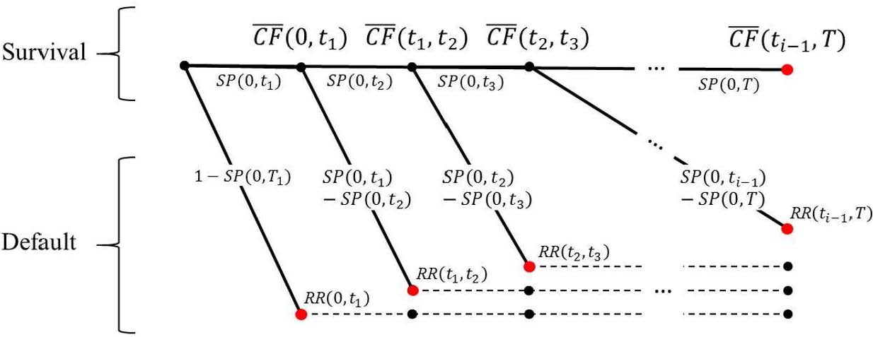
Source: Compiled by the authors.

where $\overline{CF} (t$_{i_1},t_i) is the risk-free cash-flow to be paid by the instrument; SP(0,t_i) is the survival probability of the product between t_i − 1 and t_i; 1 − SP(0,t_i) is the default probability for the same period; and RR(t_i − 1,T_i) is the estimated Recovery Rate for each period.

The tree shows that bond payments do have a survival probability at each node t_i but it is complemented by its default probability at the same node, where the payment value will only be the estimated recovery. That is to say, at every node t_i a default event can occur, or the obligor will continue until the next datet_i + 1. Following default, the non-defaulted path continues (as indicated by the upper continuation of the tree), but the defaulted security, for a given node, only earns its recovery payoff and ceases to exist (as represented by the dashed lines). The sum of the payment scenarios (red circles) weighted by the probability of their occurrence is equal to the instrument’s fair value. The above also means that the probabilities attached to the branches of the tree are only the conditional default and survival probabilities at this node as seen from t = valuation date. Hence under the above model, the defaultable bond price is:

 (9)

where $\overline{CF}$ is the default-free cash flow at each node i.

3) If the above information is not available, other possible methods of estimating a PD are using:

• The quoted CDSs spread (over bonds issued by the same counterparty with the same maturity) in a non-active market.

• The quoted YTM of bonds issued by the same counterparty with the same maturity in a non-active market.

• The quoted CDSs spread (over bonds issued by the same counterparty with similar maturity) in a non-active market. The spread should be adjusted for the difference in maturity.

• The quoted YTM of bonds issued by the same counterparty with similar maturity in an active or non-active market. The PD is adjusted for the difference in maturity.

4) If the specific counterparty does not have quoted CDSs of bonds (in active or non-active markets), the PD may also be obtained from the quoted CDSs or bonds of other companies with the same rating and characteristics (sector, country, size, etc.).

5) If the specific counterparty does not have quoted CDSs of bonds, nor a public credit rating, the entity could internally estimate a credit rating for the specific counterparty. The objective of the model that we present in the following section is to estimate that internal credit rating.

Once the credit rating is obtained, there are two possibilities for estimating the PD:

• Derive the PD from the quoted CDSs or bonds of companies with the same rating and similar characteristics (sector, country, size, etc.).

• Use the default studies published by the rating agencies (Ou et al., 2016 and Vazza et al., 2018), which show realized default rates for various rating categories and the “ratings migration” or transition matrices (see Table 2). However, this second possibility does not include forward-looking adjustments.

Table 2. Corporate 1 year default probabilities

S&P Rating	Default rate	Moody's Rating	Default rate
AAA	0.00%	Aaa	0.000%
AA	0.02%	Aa	0.024%
A	0.06%	A	0.061%
BBB	0.17%	Baa	0.202%
BB	0.58%	Ba	0.968%
B	3.41%	B	3.634%
CCC/C	24.50%	Caa-C	10.729%

Source: Ou et al. (2016) and Vazza et al. (2018).

On the other hand, as stated before, under IFRS 9 the estimation of future credit losses depends on the classification of the financial asset in three possible stages. If the financial asset is classified in stage 1, one year expected losses are estimated (i.e. one year PD is used). If the financial asset is classified in stages 2 or 3, lifetime expected losses are estimated (i.e. PD until maturity is used).

Initially, all financial asset are classified in stage 1. A financial asset is reclassified to stage 2 if there has been a significant increase in credit risk since initial recognition. If the financial asset is impaired (credit losses are incurred), the financial asset is classified in stage 3.

At each reporting date, an entity shall assess whether the credit risk on a financial instrument has increased significantly since initial recognition. When making the assessment, an entity shall use the change in the risk of a default occurring over the expected life of the financial instrument instead of the change in the amount of expected credit losses. To make that assessment, an entity shall compare the risk of a default occurring on the financial instrument as at the reporting date with the risk of a default occurring on the financial instrument as at the date of initial recognition and consider reasonable and supportable information, that is available without undue cost or effort, that is indicative of significant increases in credit risk since initial recognition (IFRS 9 paragraph 5.5.9).

IFRS 9 (paragraph B5.5.17) recognizes that a significant change in the instrument’s credit rating is a possible way to analyze if there has been a significant increase in credit risk since initial recognition. Therefore, FRS model can also be used for this.

As an exception to the stages, an entity shall always measure the loss allowance at an amount equal to lifetime expected credit losses for:

• (a) trade receivables or contract assets that result from transactions that are within the scope of IFRS 15, and that:

  • (i) do not contain a significant financing component in accordance with IFRS 15 (or when the entity applies the practical expedient in accordance with paragraph 63 of IFRS 15); or

  • (ii) contain a significant financing component in accordance with IFRS 15, if the entity chooses as its accounting policy to measure the loss allowance at an amount equal to lifetime expected credit losses. That accounting policy shall be applied to all such trade receivables or contract assets but may be applied separately to trade receivables and contract assets.

• (b) lease receivables that result from transactions that are within the scope of IAS 17, if the entity chooses as its accounting policy to measure the loss allowance at an amount equal to lifetime expected credit losses. That accounting policy shall be applied to all lease receivables but may be applied separately to finance and operating lease receivables.

3 Proposed credit model (model basics)

Our model may be called the “Financial Ratios Scoring” (FRS) model. We have developed it ourselves, and we have used it in practice during consultancy services for a wide range of companies and sectors.

The FRS model is partially based on Duan et al. (2018) and Ivanovic et al. (2015).

Its main model input is the information obtained through the counterparty financial statements (i.e. the main inputs are financial ratios). According to the values of several key balance sheet and profit and loss account ratios, the company is allocated to a certain position (score) within a consistent distribution of companies that possess an official credit rating (issued by a rating agency or quoted by relevant financial vendors), and which belong to the same or similar sectors. The position within the distribution is related to a certain credit rating (the official rating of companies with a similar score).

According to Cappon et al. (2018), credit ratings are “opinions” issued by rating agencies regarding the credit worthiness of corporate, municipal and sovereign borrowers. Agencies generally avoid claiming that credit ratings predict probabilities of default. Nevertheless, they do publish detailed default studies which show historical ratings migration and default events as a function of the initial rating and time horizon. Analysts and risk managers routinely use default study data as estimates of default probabilities. In practice, it is assumed that a rating generally matches a range of default probabilities.

The FRS model is intensive in terms of data collection (as we will see, it is necessary to create a distribution of sector companies). However:

• It can be considered to be highly consistent since the model’s inputs are calibrated with the financial information of companies which do have an agency rating.

• It is not as intensive as other similar models (see section 1).

Among the ratios considered by the model (which may also vary from one sector to another), those with higher relevance in terms of credit risk are those related to debt and interest coverage, leverage or liquidity. In other words, the relative debt level of a company is generally the factor with most influence on its credit risk. Growth and profitability are also considered, but linked to liabilities and equity.

As the FRS relies on accounting information, two possible limitations to the model are earnings manipulation, and the fact that qualitative information is not considered.

With regard to earnings manipulation, Alissa et al. (2013) identify firms that deviate from expected credit ratings, and demonstrate that these empirically estimated credit rating deviations are associated with earnings management activities. Their results suggest that firms above or below their expected credit ratings may be able to successfully achieve a desired downgrade or upgrade through the use of earnings management. Therefore, if the financial information has been manipulated, the credit rating obtained will also differ from the correct rating. Nevertheless, our model generally assumes that the financial information used is correct. The model’s main objective is not to detect possible fraudulent activity related to financial statements.

Conversely, default risk (credit risk) can generally be measured in three different ways: using quantitative data; using qualitative data; or by using a combination of both. Quantitative data includes equity prices; credit market data; financial instrument quotes other financial data, etc. Qualitative data includes the entity’s structure; how the entity is perceived by the market; business estimations; business plans; information regarding the entity’s governance and risk appetite, etc.

The model we propose uses quantitative data as its main input (financial information (financial ratios) obtained from the entity’s financial statements). In theory, we do not use qualitative data in our model, fundamentally due to the following factors:

• Qualitative factors or metrics are difficult to measure and to model due to several reasons such as the fact that the same information is not available for all entities, and they entail a significant level of subjectivity, etc. In this sense, as our model aims to be both robust and easy to implement at the same time, it does not consider qualitative factors (at least not directly).

• In recent years, financial and market information has tended to be more reliable (quantitative factors). This makes quantitative factors more effective when estimating a probability of default or assigning a credit rating. In fact, in terms of default events and recovery rates, quantitative models have been taking new assumptions into account and covering recent scenarios (for example, see Moody’s latest reports on default risk and recovery rates (Moody’s, 2017)).

It can be argued that FRS model uses forward-looking information (as required by IFRS 9). This is because, as we will further see in the following section, the obtained credit rating is calibrated using official credit ratings that are developed by official rating agencies. These official ratings are obtained by the agencies not only using quantitative information (financial statements ratios) but also using qualitative factors like: business perspectives, corporate governance, the regulatory and competitive environment, financial policy, etc.

Therefore, qualitative aspects are also covered to a certain degree. However, those aspects are not directly modelled nor measured.

Moreover, once the credit rating is obtained for a certain counterparty, the second step (obtaining the PD) can be done (as stated before) by reference to quoted CDSs of bonds. This information includes, in theory, all available market forward-looking information

If the PD is obtained using historical default rates, forward looking information should me incorporated. For example, the PD can be adapted to current macroeconomic conditions vs. conditions that existed when the data was collected.

4 Methodology, risk factor calibration and implementation

As previously stated, the FRS model is based on reflecting the position (score) of a company within a representative group of rated companies, so as to provide the company with a credit rating in line with its associated score.

With regard to this score:

• It may also be considered as a “percentile” in the model context (in fact, it is a percentile within a sectorial group). It is configured on a basis where 1 represents the worst position and 100 the best position.

• It will depend on the values of the financial ratios selected, and therefore on the position of each financial ratio within its group (hereinafter “distribution”).

The construction of the model consists of five main phases:

• Phase 1 – Definition of key financial ratios

• Phase 2 – Database and general score

• Phase 3 – Specific score for each ratio

• Phase 4 – Scoring matrix and βj calibration

• Phase 5 – Obtaining the credit rating for the company

Phase 1 – Definition of key financial ratios

In this first phase, a group of key financial ratios is defined for the sector to which the company belongs. Generally, these ratios are related to metrics such as coverage, leverage, liquidity, profitability and growth.

We propose the use of the ratios shown in Table 3 below as a general framework. These ratios are widely used by analysts (Fazzini, 2018) and by rating agencies (see Moody’s 2017b, for example), since they represent the key financial dimensions that act as drivers for a rating profile. They are easy to calculate using the financial information included in the public financial statements issued by companies.

Nevertheless, it should be noted that additional ratios could be included for specific sectors according to the nature of their business, such as Passenger Load in the commercial airlines sector, or Loan Default Rate in the banking sector, etc. As will be explained in subsequent sections, the intrinsic characteristics of a sector are disclosed when calibrating the ratio weights, hence to a certain extent the “sector” variable is covered by this methodology.

Table 3. Ratios used in the FRS model

Balance sheet / P&L - Ratio	Type of Ratio
(Liabilities - Cash & Securities)/Assets	Leverage
Retained Earnings/Liabilities	Leverage
Interest Expense/Sales	Coverage
EBITDA/Interest Expense	Coverage
Current Assets/Current Liabilities	Liquidity
Cash & Securities/Current Assets	Liquidity
Return on Assets (ROA)	Profitability
Return on Equity (ROE)	Profitability
Sales growth YoY, last 5y	Sales growth

Source: Compiled by the authors.

• “Interest expense/Sales” and “EBITDA/Interest Expense” (coverage ratios) focus on to what extent interest expenses related to debt are “covered” by income from normal business operations. The higher the interest expense in relation to sales or EBITDA, the weaker the financial position of the company. In other words, the ratio analyzes to what extent the entity generates sufficient resources in order to be able to pay the interests related to external debt.

  • In the first ratio, the higher the level, the lower the coverage (less sales income is available to pay the interest expense).

  • In the second ratio, the higher the ratio level, the higher the generated surplus (and the higher the coverage).

In general terms, the model places much importance on coverage ratios as a default event is usually understood as the situation in which a company is not able to entirely pay the short-term debt. In this sense, coverage ratios can act as signals of credit problems.

• “(Liabilities - Cash & Securities)/Assets” statically analyzes the company’s leverage level (or relative debt level). It compares the assets (that could be used to pay the debt) with the net debt (net of cash and liquid securities). The higher the ratio result, the higher the relative debt level (and the higher the credit risk).

• “Retained Earnings/Liabilities” compares the company’s result with its debt level. It analyzes the company’s leverage level more dynamically. The higher the ratio result, the lower the credit risk.

• “Current Assets/Current Liabilities” is known as working capital. Depending on the sector involved, the interpretation of the result may vary. Generally speaking, the higher the ratio, then the higher the liquidity level. Nevertheless, in the retail sector, a low ratio may be interpreted in a positive way, i.e. the entity is being financed by its suppliers (the average collection period is lower than the average payment period).

• “Cash & Securities/Current Assets” analyzes to what extent current assets are composed of liquidity (the higher the ratio level, the higher the liquidity level).

• ROA and ROE analyzes the profitability of the company. They calculate return in relation to assets (ROA), and return in relation to equity (ROE).

• “Sales growth” analyzes the growth in sales figures. Company growth can be analyzed in several ways (in terms of assets, sales, EBITDA or Net Profit among others). We have chosen sales growth given the fact that the other metrics may be biased due to the company’s activity. Sales figures are usually sufficiently isolated to be considered as a good estimate of company performance (always considering their relevancy in comparison to the abovementioned credit metrics).

Phase 2 – Database and general score

This phase consists of creating a database including a portfolio of companies (“peers”) which possess an official credit rating (issued by a rating agency), and of giving a general score to each of them.

Where possible, companies included in the database should belong to the same sector and country as the company under analysis, and should have recently been rated by a relevant credit rating agency (i.e. Moody’s, Fitch or S&P). Alternatively, given the limited number of rated companies over the sectors, the database can also be created by using the credit rating issued by Reuters or Bloomberg. The use of the Reuters or Bloomberg credit rating has the added advantage of giving a score between 0 and 100 as well as the rating. A given score level is related to a rating level.

In some cases, it can prove difficult to find peers since companies are highly diversified and act in many different industries and markets at the same time. Nevertheless, we recommend the inclusion of as many peers as possible.

A score is assigned to each peer company in the portfolio, and each company is ranked according to its position (a percentile between 1 and 100) within the entire portfolio of companies. This position represents the general score. By way of example, for a specific real case (in a specific sector), we included the information required in a database in order to build the cumulative distribution function (Figure 2).

Figure 2: Example of Score distribution per Credit Rating

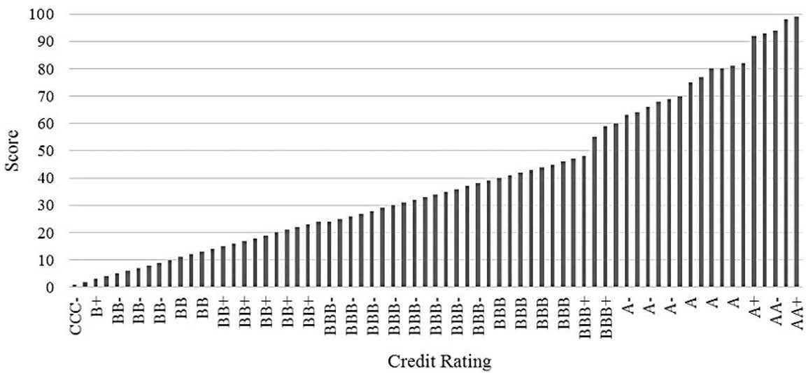
Source: Compiled by the authors.

As can be seen in the above distribution (Figure 2), the credit rating is directly related to the score (“position” or “percentile”) within the distribution. This distribution was created using Reuters. Certain companies with an equal rating are scored slightly differently according to their outlook, size and debt coverage. In the example above, this means that there are 13 companies with the same rating (BBB-) between percentile 25 and 37. This is normal given the fact that there are more companies rated between BBB- and BBB+ than in any other rating bucket. Figure 2 above represents a cumulative distribution of 63 rated companies. Its corresponding probability density function is shown in Figure 3:

Figure 3: Example of Density function of Credit Rating

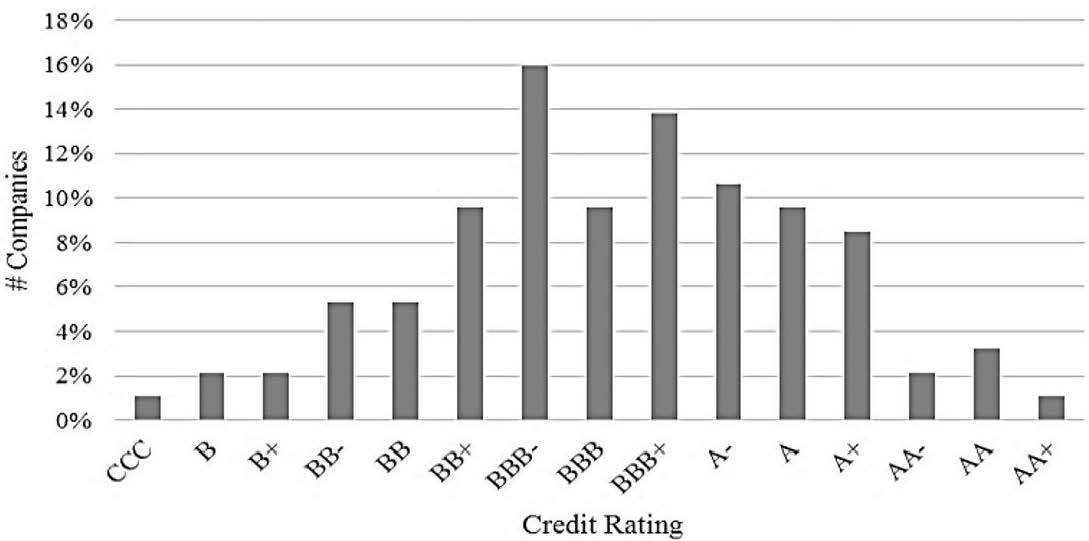
Source: Compiled by the authors.

Phase 3 – Specific score for each ratio

In this phase, we assign a score to each peer company in the portfolio in relation to each ratio. In other words, each company has on the one hand a general score (Phase 2), and on the other a specific score for each ratio (Phase 3).

Therefore:

• We calculate every ratio included in Table 3 for all of the companies in the sample.

• We create a distribution for each ratio according to the results.

• Each company is given a score (percentile) for each ratio depending on its position within the distribution.

In theory, the ratio distribution (vector) should be as granular as possible.

Phase 4 – Scoring matrix and β_j calibration

A matrix is prepared which shows the relationship between the comparable companies’ rating, their general score, and the score of each ratio. The following table presents an example:

Table 4. Example of Scoring table (general and specific scores)

Company	General Score		Score for each ratio
	Rating	General Score	ROE	ROA	Interest coverage	Net Debt / Assets	Etc.
Company A	BBB-	25	37	40	28	48
Company B	BBB+	52	65	61	54	65
Company C	BB+	16	12	7	20	22
Company D	A	80	60	42	84	64
…	…	…	…	…	…	…	…
Company n	BB+	13	6	1	16	4

Source: Compiled by the authors.

The above matrix (Table 4) should be fed with the following inputs:

• The name of each peer company in the portfolio.

• The rating and general score of each peer company in the portfolio.

• The specific score of each peer company in the portfolio for each ratio.

We can also obtain a score for each ratio for the company under analysis (using the previous distribution). The question is how we can use the scores for each ratio for the company under analysis in order to assign a general score for that company (and, therefore, a rating).

The first item to be calculated is the representativeness of each ratio within the rating assigned to each company, i.e. to what extent the score of each ratio influences the general score. We know that the ratios used do not entirely cover the wide range of risk factors considered by rating agencies (although they do implicitly include qualitative factors). Given the nature of our analysis, it is clear that the overall credit score is a dependent variable, and that the ratios’ scores are the independent variables, assuming there are risks not covered in the model. From our previous practical research (see also the empirical text in the following section), it can be concluded that the use of an Ordinary Least Squares methodology to calibrate a linear regression represented by a weighted sum of the ratios scores gives highly accurate results in terms of the model’s goodness of fit. In other words, we are able to estimate the overall credit score of a company as follows:

$$Score_{company_{i}} = \sum_{j=1}^{n} Score_{company_{j}} \beta_{j}$$   (10)

Where β_j is the coefficient assigned to the ratio _j. β_j is calculated using the database of companies already created. By way of example, we use the data included in Table 5 (an example of a Scoring Matrix) in order to calibrate each β_j for a given sector:

Table 5. Scoring table to be used as an example

Company	General Score		Score for each ratio
	Rating	General Score	Profitability ratio	Leverage ratio	Coverage ratio	Liquidity ratio	Growth ratio
Company A	BB+	15	2	29	14	53	38
Company B	BBB+	61	10	64	55	31	72
Company C	BBB-	37	12	24	54	48	33
Company D	BBB+	53	86	12	62	25	95
Company E	BBB-	24	61	13	52	5	84
Company F	BBB+	60	84	37	59	28	62
Company G	BBB-	25	5	6	44	19	94
Company H	BBB	45	8	97	14	79	14
Company I	BB+	22	46	16	39	16	59
Company J	BBB+	58	80	42	70	49	58
Company K	B	2	19	1	22	1	29
Company L	BBB-	24	65	13	48	26	45
Company M	BBB-	25	38	19	18	29	4
Company N	BBB+	60	29	48	63	51	14
Company O	BBB-	30	6	45	40	28	21
Company P	A	91	51	83	95	62	90

Source: Compiled by the authors.

Following a Least Squares methodology, the following β_j⁵are obtained with regards to (10):

Table 6. β_jcalibration for (3) with data set of Table 5

Profitability	Leverage	Coverage	Liquidity	Growth
β1 = 5.45%	β2 = 42.27%	β3 = 48.03%	β4 = 3.25%	β5 = 1.00%

Source: Compiled by the authors.

The linear regression and the R² for the previous calibration are shown below. The representativeness and goodness of fit of the model are sufficiently satisfactory to be able to consider the model as consistent, as no high multicollinearity is found. It should be noted that not all sectors fit equally in a linear model, and the dependency on the database size and on certain ratios is relatively moderate. The analyst should select the sectorial ratios which best represent the credit performance.

Figure 4: Example of Linear regression plot for the FSR model example

Source: Compiled by the authors.

The representativeness and goodness of fit of the model appear to be consistent with general market ratings.

Phase 5 – Obtaining the credit rating for the company

Once the β_j are obtained, two different methodologies can be applied so as to assign a general score (and therefore a credit rating) to the company under analysis.

The first methodology consists of applying the model as (3) in order to obtain the general score of the company. If, for example, we consider that the company (the counterparty) analyzed has the following ratio scores:

Table 7. Ratio Scores of the analyzed company

Profitability	Leverage	Coverage	Liquidity	Growth
24	19	38	32	56

Source: Compiled by the authors.

then the model gives a score of 29.19, which means a BBB- rating in line with the score distribution shown in Figure 1.

The second methodology consists of applying a solution to the model based on a difference-simulation methodology, which in turn covers the root mean square error as far as is possible, which in this example was 6.25. That is to say, while taking into account the existing convexity in the relationship between a company’s general score and its implied credit rating, we propose that the weighted sum of differences between the analyzed company’s ratio scores and those of each comparable company should be computed. Firstly we obtain the distance between the analyzed company and the comparable company. Thus the simulated company score will be equal to the sum of the weighted sum of differences and the current comparable company score.

$$Score_{company|comparable_{i}} = \left\lbrack \sum_{j = 1}^{n} (Score_{Company \ ratio_{j}} - Score_{Comparable_{i} \ ratio_{j}} ) \beta_{j} \right\rbrack + Score_{comparable_{i}} $$   (11)

This is carried out in order to capture the actual difference between our computed rating and the theoretical rating that the analyzed company would have if a starting point were taken. That is, we compute the weighted difference based on the calibrated β_j but, by applying the difference to the actual score of the comparable company, we place the analyzed company in a score according to a central point. In this way, the regression error is covered to a certain degree. Each result may be considered as a simulation. The average of simulations will represent the company’s score. The simulation plot can be seen below, and retrieves a concentration above a score of 32 (BBB-), with an average of 31.76 and a median of 32.84. This method also provides us with an estimate as to the range in which the score can be placed. It would obviously be necessary to include many more companies in the database in order to perform a consistent simulation, but for the sake of clarity, this example has been carried out from the sample listed in Table 5.

Figure 5: Company score simulations performance

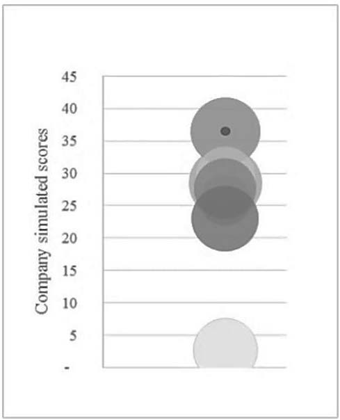
Source: Compiled by the authors.

5 Empirical test

So as to assess the accuracy of the model proposed, we have selected several companies within a given sector in order to apply the model to them. The outcome is expected to be equal to the overall ratings, or much closer to those provided by the market.

The chosen sector is “Global Surface Transportation and Logistics”. This sector needs some further ratios to be added to those detailed in Section 3. In fact, certain ratios need to be eliminated in order to avoid multicollinearity issues or betas near to zero.

The ratios added are detailed below. They improve the financial representativeness within the model since they are expected to explain particular characteristics of the sector (Moody’s (2017c) and Moody’s (2017d)):

• Profitability, measured by pre-tax income as a percentage of sales. It provides a metric on the company’s effectiveness with regard to the cost structure and its capability to reach yield premiums in comparison with peer companies. The capital-intensive nature of the transportation industry makes it important to include interest expense when considering profitability, as capital costs are as relevant as operating costs. Therefore, while this ratio may be relevant for modelling purposes, correlation and significance should also be checked.

• Financial leverage and coverage metrics are indicators of a company’s financial capacity and long-term viability. Financial flexibility is critical to this sector as it indicates the degree of stress a company would suffer during an economic downturn. In addition, leverage affects a company’s ability to reinvest in the business, as a highly leveraged company may not have the same access to capital (new funds) as other companies with a lower leverage level. Furthermore, leverage partly affects the capacity to deal with changing market conditions in the highly cyclical business operations to which this type of company may be exposed. Financial leverage and coverage are additionally represented in the model by the following ratios:

  • Debt/EBITDA ratio is an indicator of debt serviceability and leverage, and is commonly used in this sector as a proxy for comparative financial strength.

  • Funds from Operations (Free Cash Flows from Operations minus Capex) to Debt is an indicator of a company’s ability to repay principal on its outstanding debt. This ratio compares cash flow generation from operations before working capital movements to outstanding debt.

  • EBIT to Interest Expense is an indicator of a company’s ability to cover its ongoing costs of borrowing.

Other ratios specifically related to airlines (e.g. Passenger Load) were also candidates for inclusion, but were finally discarded since the database created is heterogeneous in terms of the transportation sector.

In this way, we constructed a wide data set of companies belonging to the “Global Surface Transportation and Logistics” sector for which overall ratings are issued by Reuters. We have computed the following ratios and the inherent percentile within the sample for each company and ratio: Pre-tax Income to Sales; Debt to EBITDA; Funds from Operations to Debt; EBIT to Interest Expense; Return On Equity; Net Margin; Return On Assets; EBITDA to Interest Expense; Debt to Equity; Debt to Assets, Cash to Total Debt; Short Term Debt to Total Debt; and Quick Ratio.

The following companies were finally chosen from the sample in order to calibrate the model factors, since they possess the most liquid, updated financial information in line with the financial statements date used (31/12/2015). All of these companies do not exactly move in the same business lines or even in the main sector. However, one should consider the fact that only including companies fully matching in terms of size, sector and business lines can make the model calibration poor as there exist very few companies exactly equal, concerning the above requirements. Therefore, it has been necessary to widen the sample with similar companies although they do not fully match each other regarding all their business lines or their inherent nature. What we have been looked for is the construction of a consistent sample with as many similar companies as possible taking into consideration the number of companies with ratio distribution information on financial data bases and vendors (e.g. Reuters). In terms of explanatory capacity, most of these companies are similar to the initial sample ones:

Table 8. Sector companies used to test the FRS model

Company Name	Reuters Rating (31/12/2015)
A P MOLLER - MAERSK 'A'	BBB
AEGEAN AIRLINES CR	BBB+
AIR FRANCE-KLM	B+
EASYJET PLC	AA-
WIZZ AIR HOLDINGS PLC	A+
FRAPORT AG	BBB+
FLUGHAFEN ZUERICH AG	A+
HAMBURGER HAFEN UND LOGISTIK AG	BBB
AENA SME SA	A-
VINCI.SA	BBB+
EIFFAGE SA	BBB
HAPAG LLOYD AG	BB
VTG AG	BB-
KONINKLIJKE VOPAK NV	BBB-
OESTERREICHISCHE POST AG	AA-
POST NL NV	BB+
PANALPINA WELTTRANSPORT HOLDING AG	A+
KUEHNE UND NAGEL INTERNATIONAL AG	AA+
CEVAL LOGISTICS AG	B
BBA AVIATION	BBB
BPOST	AA
DEUTSCHE LUFTHANSA (XET)	BBB
DEUTSCHE POST (XET)	BBB+
DSV 'B'	A+
FIRST GROUP	BBB
INTL.CONS.AIRL.GP.(CDI)	BB
IRISH CONT.GP.UNT.	AA-
ODET (FINC DE L')	BBB-
SIAS	BB+

Source: Reuters.

The following figure shows the general and particular percentiles for each sample company and ratio within the sectorial database used:

Table 9. Sector companies and their ratio percentiles from the sample

Company Name	Reuters Rating (31/12/2015)	Overall percentile	PreTax Income / Sales	Debt / EBITDA	Funds from Ops / Debt	EBIT / Int. Expense	ROE	Net Margin	ROA	Int. Coverage	D/E Ratio	D/A Ratio	Cash/ Total Debt	Short Term Debt/ Total Debt	Quick Ratio
A P MOLLER - MAERSK 'A'	BBB	44	24	36	27	61	6	24	18	64	67	64	82	67	61
AEGEAN AIRLINES CR	BBB+	76	67	15	85	82	82	67	82	79	70	82	85	30	73
AIR FRANCE-KLM	B+	4	6	76	18	12	100	3	3	39	0	30	48	21	9
EASYJET PLC	AA-	92	73	18	67	88	70	76	85	88	73	79	79	9	24
WIZZ AIR HOLDINGS PLC	A+	90	76	12	88	85	88	85	97	82	85	88	91	97	79
FRAPORT AG	BBB+	47	79	70	45	30	21	73	30	21	36	21	27	48	30
FLUGHAFEN ZUERICH AG	A+	90	94	45	73	67	24	91	52	70	61	58	52	91	100
HAMBURGER HAFEN UND LOGISTIK AG	BBB	45	70	39	58	48	45	58	45	55	52	61	55	61	91
AENA SME SA	A-	65	97	82	64	42	67	97	61	48	12	9	12	55	12
VINCI.SA	BBB+	68	61	85	61	45	52	52	36	33	33	48	0	33	33
EIFFAGE SA	BBB	36	36	94	24	18	36	21	15	6	6	12	33	24	48
HAPAG LLOYD AG	BB	12	9	79	6	9	3	9	12	9	45	39	24	36	15
VTG AG	BB-	8	18	91	21	3	12	18	6	3	9	0	6	85	42
KONINKLIJKE VOPAK NV	BBB-	33	100	61	52	39	58	94	64	42	27	18	9	88	64
OESTERREICHISCHE POST AG	AA-	92	27	6	94	91	42	33	58	94	88	94	94	3	76
POST NL NV	BB+	23	55	48	55	36	0	42	76	24	97	27	45	100	45
PANALPINA WELTTRANSPORT HOLDING AG	A+	90	15	3	97	94	55	12	67	97	94	100	100	0	85
KUEHNE UND NAGEL INTERNATIONAL AG	AA+	99	39	0	100	97	79	36	88	91	91	97	97	6	58
CEVAL LOGISTICS AG	B	2	0	100	9	0	97	0	0	0	100	3	21	79	52
BBA AVIATION	BBB	43	33	33	70	24	9	45	24	36	76	76	76	94	97
BPOST	AA	98	88	9	91	100	91	79	94	100	82	91	88	42	67
DEUTSCHE LUFTHANSA (XET)	BBB	42	45	42	33	64	76	48	70	61	39	67	61	15	18
DEUTSCHE POST (XET)	BBB+	64	21	30	42	73	61	30	55	73	58	73	67	64	55
DSV 'B'	A+	90	42	27	76	58	64	39	79	52	64	70	70	82	82
FIRST GROUP	BBB	41	12	64	12	15	18	15	21	18	30	36	30	76	36
INTL.CONS.AIRL.GP.(CDI)	BB	11	58	52	30	52	73	61	73	58	15	45	64	52	27
IRISH CONT.GP.UNT.	AA-	94	82	24	79	76	94	88	100	76	55	55	42	18	70
ODET (FINC DE L')	BBB-	35	64	88	0	55	30	64	39	45	48	52	36	12	39
SIAS	BB+	26	91	73	39	33	33	82	33	30	18	15	39	73	94

Source: Compiled by the authors; Reuters.

It should be highlighted that the overall percentile for each company was assigned by a random number within a confidence interval of percentile for its rating, in order to test the capacity of the model to cover the existing percentile dispersion within the same notch (which may at times result in rating down/upgrades), particularly for ratings from BB+ to BBB+, as explained below.

Testing the sample distribution:

The randomness upon which a company overall percentile may vary was applied by using the following sample distribution:

Figure 6: In - sample distribution function

Source: Compiled by the authors; Reuters.

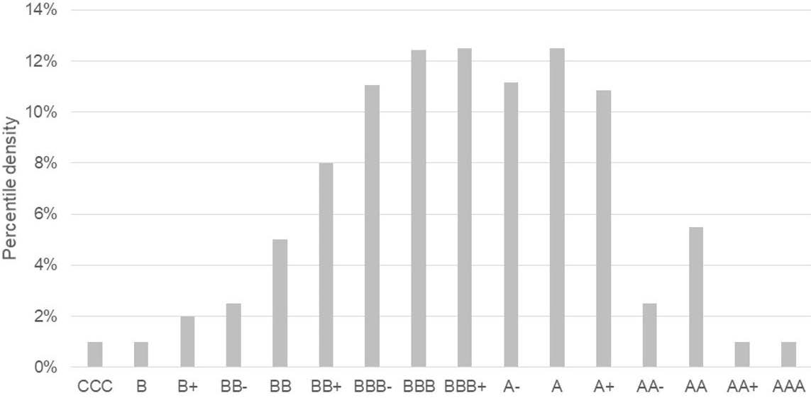
It is assumed that the percentile distribution follows a normal distribution function, therefore the average expected dispersion within each rating notch has been applied following a normal distribution. The figure below shows a sample of the simulation⁶ for the initial percentile of each company:

Figure 7: Percentile dispersion simulation from Probability Density Function

Source: Compiled by the authors.

It may be noted that generally speaking, higher dispersion occurs in notches near to non-investment grade letters or below, with both the highest investment grades and highly speculative grades/defaulted remaining almost unchanged, as expected according to the most recent average migration matrices:

Table 10. 2017 One-Year Letter Rating Migration Rates

From\To	AAA	AA	A	BBB	BB	B	C/Default
AAA	100.00%	0.00%	0.00%	0.00%	0.00%	0.00%	0.00%
AA	0.00%	79.80%	20.20%	0.00%	0.00%	0.00%	0.00%
A	0.00%	1.35%	94.44%	3.89%	0.24%	0.00%	0.08%
BBB	0.00%	0.06%	2.88%	95.48%	1.29%	0.29%	0.00%
BB	0.00%	0.00%	0.00%	6.74%	88.93%	3.97%	0.36%
B	0.00%	0.00%	0.00%	0.10%	7.24%	86.92%	5.75%
C/Default	0.00%	0.08%	0.00%	0.00%	0.08%	4.99%	94.86%

Source: Moody’s; compiled by the authors.

Certain specific percentile simulations were tested with the following results:

Table 11. Simulated vs historical notch migration probability

Company	Reuters Rating	Simulated notch migration probability	Historical notch migration probability
POST NL NV	BB+	19.4%	14.24%
KONINKLIJKE VOPAK NV	BBB-	9.7%	13.49%
AENA SME SA	A-	14.3%	13.28%

Source: Reuters; Moody’s; compiled by the authors.

Thus we can assume that the distribution used, built upon the overall percentile distribution as taken from Reuters, is reliable for modelling purposes.

Once the overall percentile distribution taken from the sectorial sample is found to be correct, the percentiles for all the ratios are computed, and the betas are calibrated under OLS following the abovementioned methodology. Firstly, as mentioned in footnote 4, the model is calibrated without boundaries so as to check statistical strength and eliminate non-significant variables. Thus many of the ratios previously defined in Phase 1 are eliminated given the multicollinearity in the regression, since there are high correlations (measured in differences to avoid stationarity issues) between them and the new explanatory ratios. No relevant information from certain other ratios is added to the model for this particular sector (betas in the regression are near to 0 or negative due to the inverse correlation and non-significance).

Thus in this case, Funds from Ops to Debt and EBIT to Interest Expense are found to be the ratios with relevant statistical significance (95% confidence, 13 degrees of freedom) as follows

Table 12. Significance statistics for the main ratios

Ratio	p-value	t-statistic
Funds from Ops / Debt	0.0057	3.218
EBIT / Interest Expense	0.0471	2.169

Source: Compiled by the authors.

while Pretax Income/Sales, Debt EBITDA Debt/Assets are the variables with residual explanatory strength. The correlation matrix presented below helps to explain the multicollinearity issues to be avoided:

Figure 8: Ratio percentiles’ correlation matrix (measured in differences)

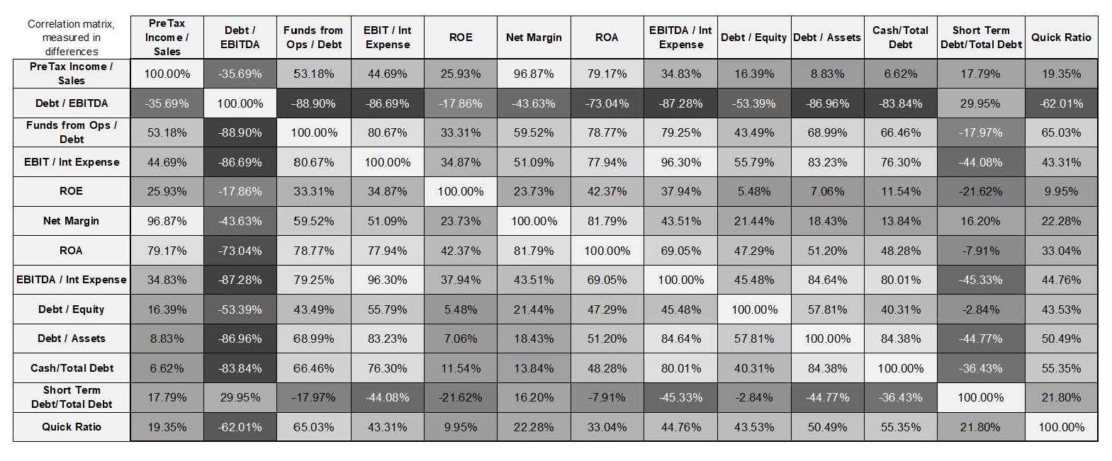
Source: Compiled by the authors.

Meanwhile, the regression betas with no boundaries with the most explanatory variables are as follows:

Table 13. Ratios and their corresponding calibrated betas for the tested sector

Pretax Income / Sales	Debt / EBITDA	Funds from Ops / Debt	EBIT / Int Expense	Debt / Assets
-0.662%	2.192%	50.389%	51.484%	1.342%

Source: Compiled by the authors.

The homoscedasticity, multicollinearity and normality in residuals have been also analyzed with the following results:

• Multicollinearity:

Table 14. R2 and VIF for the two significant explanatory variables

R2 for significant exogenous var.	Variance Inflation Factor
59%	2.51

Source: Compiled by the authors.

• Homoscedasticity: Breusch-Pagan test outcome with a p-value = 0.897.

• Normality in residuals: Jarque-Bera test with a p-value > 0.70 with 100,000 simulations. Although the sample is relatively small, we also get the following QQ plot:

Figure 9: QQ Plot for normality test in regression residuals

Source: Compiled by the authors.

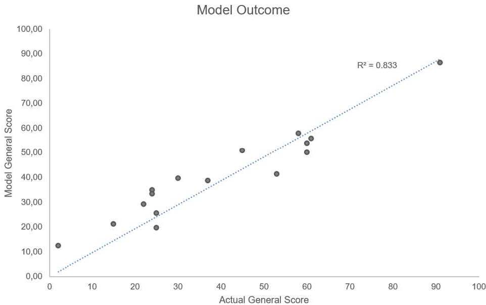
Hence the calibration provides an R² of 83.22% between the actual percentile for each company and the one simulated:

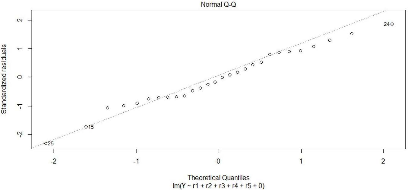
Figure 10: Regression plot (Modelled vs Actual percentiles)

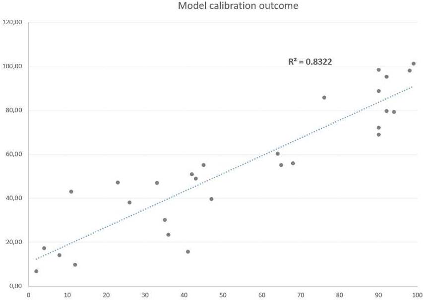
Source: Compiled by the authors.

The previous calibration provided a sum of betas equal to 104.75%. If the boundaries for making the sum of betas equal to 100% are applied, the results are almost unchanged:

Table 15. Ratios and their corresponding calibrated betas for the tested sector, with boundaries

Pretax Income / Sales	Debt / EBITDA	Funds from Ops / Debt	EBIT / Int Expense	Debt / Assets
0.000%	0.293%	50.196%	49.201%	0.310%

Source: Compiled by the authors.

R² in this case remains almost the same: 83.07%.

In order to check the goodness of fit added to the model when including the new explanatory variables, we also calibrated the model with the standard ratios as defined in Phase 1. The results are shown below:

Table 16. Standard ratios and their corresponding calibrated betas for the tested sector, with boundaries

Net Margin	ROA	EBITDA / Int. Expense	Debt / Equity	Debt / Assets	Quick Ratio
7.59%	22.06 %	33.86%	0.23%	22.08%	10.17%

Source: Compiled by the authors.

with Return on Equity, Cash to Total Debt and Short-Term Debt to Total Debt with null explanatory strength in any of the local minimums found when calibrating the model.

Figure 11: Regression plot (Model vs Actual percentiles), Standard ratios

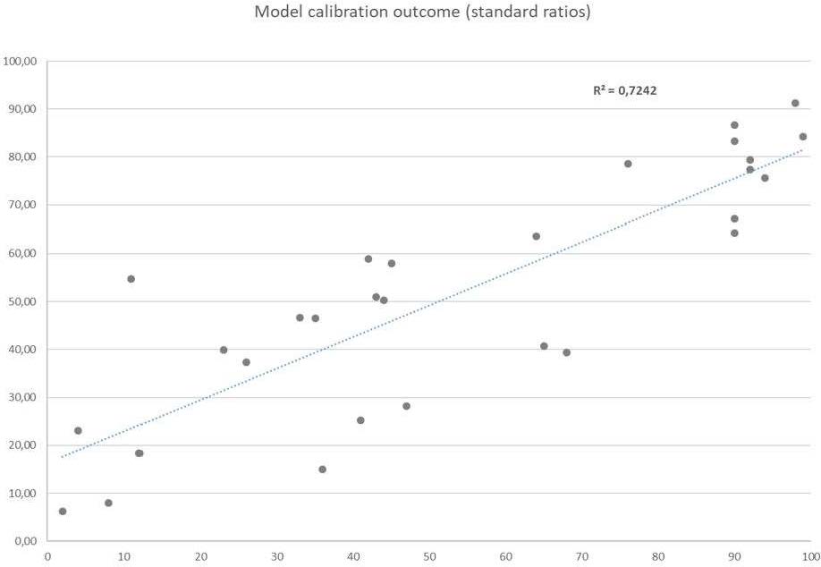
Source: Compiled by the authors.

As can be seen, once specific-sectoral ratios are used, the explanatory capacity added to the model is boosted by at least 11% (increasing from an R² of 72% to 83%).

It should be noted that including the whole set of ratios (general + sector-specific) in the regression model only increases the explanatory power from 83% to 87.92%. However, the multicollinearity added to the model is huge. Hence, the idea of using sector-specific ratios to build the model is assumed as the basis for this kind of models.

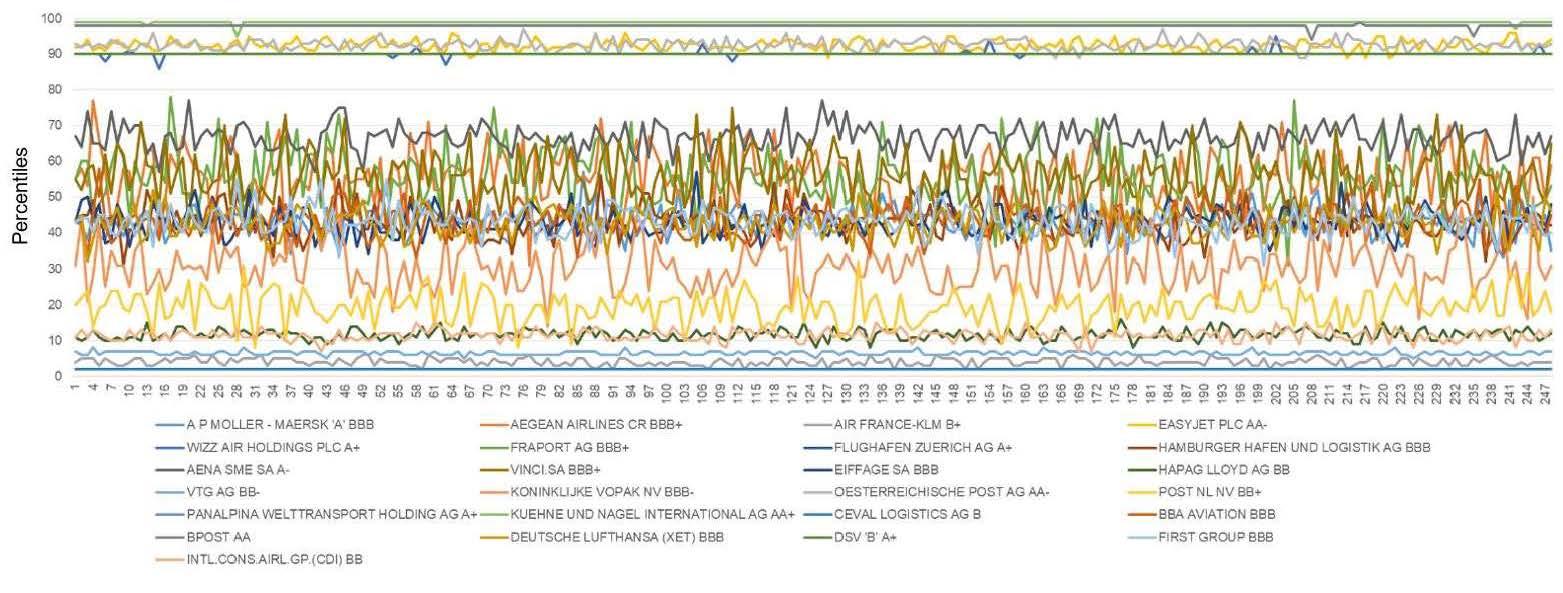
The model calibration captures the amount and direction of trend changes for each company percentile in general terms, with a correlation measured in levels and in differences higher than 90%. Hence the financial hypotheses carried out for the sector outperform regular ratios:

Figure 12: Actual percentiles vs simulated percentiles for the sample chosen

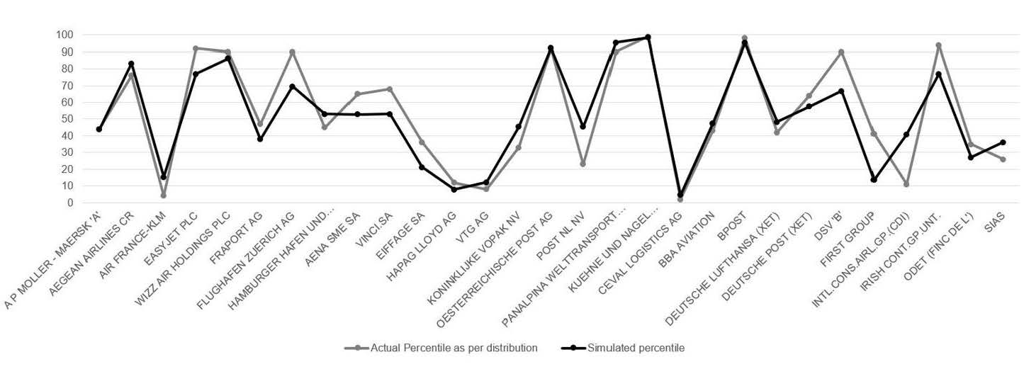
Source: Compiled by the authors.

Official Rating vs model rating

The following table compares the model’s rating for companies with agency and vendor ratings:

Table 17. Comparison between FRS model outputs, agency ratings and Reuters rating (31/12/15)

Company	Agency Rating	Reuters Rating	Model Rating	Model – Agency deviation
A P MOLLER - MAERSK 'A'	BBB+	BBB	BBB	One notch
DEUTSCHE LUFTHANSA (XET)	BBB-	BBB	BBB	One notch
POST NL NV	BBB-	BB+	BBB	One notch
EASY JET PLC	BBB+	AA-	BBB+	-
VINCI SA	A-	BBB+	BBB+	One notch
FIRST GROUP	BBB-	BBB	BBB-	-

Source: Moody’s; S&P; Reuters; compiled by the authors.

Out-of-sample testing:

In order to test the predictive ability of the model, we randomly selected 4 companies belonging to the tested sector possessing an overall percentile published in Reuters, and we applied the model to them once the financial ratios and their percentiles were computed:

Table 18. Tested companies and their ratio percentiles from the sample

Company	Reuters Rating (31/12/2015)	Actual Percentile as per distribution	PreTax Income / Sales	Debt / EBITDA	Funds from Ops / Debt	EBIT / Int Expense	ROE	Net Margin	ROA	EBITDA / Int. Expense	Debt / Equity	Debt / Assets	Cash/ Total Debt	Short Term Debt/ Total Debt	Quick Ratio
NATIONAL EXPRESS	BBB+	52	48	58	48	27	48	55	48	27	42	42	15	58	0
NORWEGIAN AIR SHUTTLE	BB	9	3	97	3	6	27	6	9	15	3	6	18	39	6
ROYAL MAIL	A	82	30	21	82	79	15	27	27	85	79	85	58	45	21
STOLT-NIELSEN	BB+	21	52	67	15	21	39	70	42	12	21	24	3	27	3

Source: Compiled by the authors.

The results obtained when using the sectorial calibration are shown below:

Figure 13: Actual percentiles & ratings vs Simulated percentiles & ratings for the tested companies

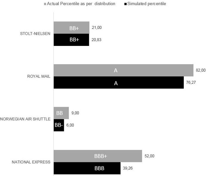
Source: Compiled by the authors.

As can be seen, the model’s ability to predict the expected rating, in this case as quoted by Reuters, can be considered to be reliable. The sensitivity of the outcomes to the percentile distribution and its link to several rating letters (e.g. Norwegian Air Shuttle) should be noted. However, in the majority of cases, the difference between the actual rating and the model rating is null or only one notch. Therefore, it does allow a link to be made between a given rating and the PDs quoted by rating agencies or financial vendors for the purpose of IFRS 9 impairment computation.

6 CONCLUSION

Under the IFRS 9 impairment model, entities must estimate the probability of default for all counterparties from fixed rate financial assets (loans, receivables, bonds, etc.) and other elements not measured at fair value through profit or loss. There are several means of obtaining the corresponding PD and generally speaking, banks and other large companies have developed internal methodologies.

In other cases, however, entities face difficulties in assigning a PD to certain counterparties due to the lack of market information concerning the counterparty; to the lack of internal or external historical default information; and to the lack of a scoring model.

In this paper, we propose a model for such cases (Financial Ratios Scoring – FRS) for which we have detailed 5 steps or phases. Fundamentally it consists of assigning a score to the counterparty according to its key financial ratios. The score places the counterparty on a percentile within a previously constructed sector distribution using companies with an official credit rating.

As we have seen, the model has several advantages:

• The only information needed for the counterparty is financial information (financial ratios) that can be obtained from financial statements.

• The database to be constructed is relatively small as compared to databases required by equivalent models.

• The model output is calibrated with market information (official credit ratings issued by rating agencies or financial vendors). Therefore, it somehow incorporates forward-looking information. Moreover, if quoted CDs of bonds are used for obtaining the PD (in a second step) updated market information is used.

• The model is relatively easy to implement.

Regarding the first of the abovementioned advantages, it should be noted that the information obtained from the counterparty’s financial statements may not be of use if it is very old, or if an event has occurred (general or specific) since the date of the financial statements which may have changed the counterparty’s creditworthiness.

The results of the empirical test performed show that the model works when certain information is available, and that the β_j coefficients are able to explain the general score with a high degree of confidence.

Moreover, it should be outlined the necessity for model monitoring and control. Due to the fact that reported information and therefore, percentile distribution could change over time. Reporting events affect the financial information so that ratios and figures change, so that the model should be reviewed and recalibrated frequently. Also, databases should be monitored, as companies’ business and structure may change as they try to adapt to business and economic conditions, including mergers, divestments, economic downturns, etc. Subsequently, the model user should monitor the explanatory variables in terms of representativeness and even include new ones if the business structure requires new metrics.